
Journal of Bioanalysis & Biostatistics
Download PDF
Research Article
*Address for Correspondence: Mark Chang, Department of Biostatistics, Boston University, Boston, Massachusetts, USA, E-mail: mychang@bu.edu
Citation: Chang M, Balser J. Adaptive Design - Recent Advancement in Clinical Trials. J Bioanal Biostat 2016;1(1): 14.
Copyright © 2016 Chang M, et al. This is an open access article distributed under the Creative Commons Attribution License, which permits unrestricted use, distribution, and reproduction in any medium, provided the original work is properly cited.
Journal of Bioanalysis and Biostatistics | Volume: 1, Issue: 1
Submission: 11 March, 2016 | Accepted: 09 June, 2016 | Published: 17 June, 2016
 Error-spending approach solved the practical problems with GSD about IA schedule, but the maximum sample size in a GSD may not be larger enough when the treatment effect is over-estimated. If we use a larger maximum sample size in GSD, it may not be costeffective. The sample size re-estimation design is developed to handle the situation when there is a great uncertainty about treatment effect, but we don’t want to make a large, unnecessary commitment before seeing the interim data.

Adaptive Design - Recent Advancement in Clinical Trials
Mark Chang1,2*and John Balser1
- 1Veristat, Southborough, Massachusetts, USA
- 2Department of Biostatistics, Boston University, Boston, Massachusetts, USA
*Address for Correspondence: Mark Chang, Department of Biostatistics, Boston University, Boston, Massachusetts, USA, E-mail: mychang@bu.edu
Citation: Chang M, Balser J. Adaptive Design - Recent Advancement in Clinical Trials. J Bioanal Biostat 2016;1(1): 14.
Copyright © 2016 Chang M, et al. This is an open access article distributed under the Creative Commons Attribution License, which permits unrestricted use, distribution, and reproduction in any medium, provided the original work is properly cited.
Journal of Bioanalysis and Biostatistics | Volume: 1, Issue: 1
Submission: 11 March, 2016 | Accepted: 09 June, 2016 | Published: 17 June, 2016
Abstract
In the past decade, the pharmaceutical industry experienced a paradigm shift from classical to adaptive clinical trial design. The high NDA failure rate and the increasing cost in pharmaceutical R & D is the motivation behind the innovation. Biostatisticians in collaboration with physicians and other major stockholders in pharmaceutical R & D are the driving force in this revolution. In this review paper, we provide an overview of adaptive trial design, covering majority of types of adaptive designs, and the opportunities, challenges, and controversies surrounding adaptive trials. We cover the topic broadly as there have been explosions of research papers that consider adaptive design over the past decade. Adaptive designs have become very popular, making it impossible to cover them all in a single overview paper.Keywords
Adaptive clinical trial; Adaptive design; Winner design add-arm design; Adaptive randomization; CRM; Sample-size reestimation; Group sequential design; Error-spendingAdaptive Design Methods in Clinical Trials
Investment in pharmaceutical research and development (R & D) has more than doubled in the past decade. The increase in spending for biomedical research does not reflect an increased success rate of pharmaceutical development. There are several critical areas for improvement in drug development. One of the obvious areas for improvement is the design, conduct, and analysis of clinical trials. Improvement of the clinical trials process includes [1] the development and utilization of biomarkers or genomic markers [2], the establishment of quantitative disease models, and [3] the use of more informative designs such as adaptive and/or Bayesian designs. We should not use the evaluation tools and infrastructure of the last century to develop this century’s advances. Instead, an innovative approach using adaptive design methods for clinical development must be implemented.In general, an adaptive design consists of multiple stages. At each stage data analyses are conducted and adaptations take place based on pdated information to maximize the probability of success of a trial. An adaptive design is a clinical trial design that allows adaptations or modifications to aspects of the trial after its initiation without undermining the validity and integrity of the trial [1-3].
The adaptations may include, but are not limited to, (1) group sequential designs, (2) sample-size adjustable designs, (3) pickthe- winner and add-arm designs, (4) adaptive treatment allocation designs, (5) adaptive dose-escalation designs, (6) biomarker-adaptive designs, (7) adaptive treatment-switching designs, (8) adaptive dose-finding designs, and (9) adaptive error-spending designs. An adaptive design usually consists of multiple stages. At each stage, data analyses are conducted, and adaptations are taken based on updated information to maximize the probability of success.
An adaptive design must preserve the validity and integrity of the trial. The validity can be classified as internal and external. Internal validity is the degree to which we are successful in eliminating confounding variables and establishing a cause-effect relationship (treatment effect) within the study itself. External validity is the degree to which findings can generalize to the population at large. Integrity involves minimizing operational bias; creating a scientifically sound rotocol design; adhering firmly to the study protocol and standard perating procedures (SOPs); executing the trial consistently over time and across sites or country; providing comprehensive analyses of trial data and unbiased interpretations of the results; and maintaining the confidentiality of the data.
Background
The term “adaptive design” in clinical trial may have been first introduced by Bauer as early as 1989 [4-8]. Adaptive Randomization designs were early studied by Hoel, Simon and Weiss, Simon, Wei, Wei & Durham, Hardwick and Stout, Rosenberger & Lachin, and more recently by Rosenberger & Lachin, Rosenberger and Seshaiyer, Hu, and Ivonova under different names [9-20]. The recent developments in adaptive randomization were covered in the book edited by Sverdlov [21]. Bayesian adaptive dose-escalation design was first studied by O'Quigley, Pepe and Fisher [22]. Chang and Chowstudied a hybrid approach with adaptive randomization [1]. Adaptive dose-escalation and dose-finding design were further studied by vanova & Kim, Yin & Yuan, and Thall [23-25]. Winner design with three groups [26] and drop-loser and add-arm designs [27] were also developed for later stage trial designs.
A randomized concentration-controlled trial (RCCT) is one in which subjects are randomly assigned to predetermined levels of average plasma drug concentration. The dose adaptation takes place based upon observed concentrations that are used in each patient to modify the starting dose to achieve the pre-specified randomized concentration. The RCCT is designed to minimize the inter individual pharmacokinetic (PK) variability within comparison groups and consequently decrease the variability in clinical response within these groups [28,29].
Adaptive methods were further developed to allow sample size reestimation [30-32], which has caused controversies surrounding the unequal weights for patients from different stages and efficiency of the design compared to GSD [33].Biomarker utilization in clinical trial was studied by Simon & Maittournam, Mandrekar & Sargent, Weir & Walley, Simon, and Baker et al. [34-38]. Population Enrichment design and adaptive designs using biomarker or genomic markers are adaptive designs that allow us to select target population based on interim data [39]. Simon & Wang and Freidlin, Jiang & Simon studied a genomic signature design, Jiang, Freidlin & Simon proposed Biomarkeradaptive threshold design, Chang and Wang, Hung & O'Neill studies population enrichment design using biomarker, which allow interim decision on the target population based on power or utility [40-45]. Song & Pepe studied markers for selecting a patient's treatment [46]. Further studies on biomarker-adaptive design were done by Beckman, Clark, and Chen for oncology trials, and more recently by Wang, Wang, Chang, and Menon using a two-level relationship between biomarker-primary endpoint [47-50].
Recently, adaptive design has been developed into multiregional clinical trials [51], in which sample size can be redistributed among different regions depending on the interim data in different regions to maximize the probability of success.
For any particular compound, there are many adaptive designs can be used. The optimal design fits particular needs should be based on so-called evaluation matrix. Menon and Chang studied the optimization of the adaptive design was using simulations [52]. Chang provides a practical approach [53]. For adaptive trial interim data monitoring and adaptation-making, readers can refer to books Proschan, Lan, and Wittes, DeMets, Furberg, and Friedman, and Chang [54-56].
Recent analysis and applications
The analyses of data from adaptive trials are complicated with many unsolved controversies, provoking discussions of fundamental statistical principles or even scientific principles in general [57,58]. Different proposed methods have been studied by Chang, Emerson, Liu and Hall, Lui and Xiong, Chang, Chang, Wieand, and Chang, Chang, Gould, and Snapinn, and Pickard and Chang [59-71].
In a recent investigation on the use of adaptive trial designs [72], it is reported that among all adaptive design they investigated, 29% is GSD, 16% SSR, 21% Phase-I/II or Phase-II/III seamless designs, and 41% dose-escalation, dose-selection and others.
The adaptive design has gained popularity since 2005 when a group of people from the pharmaceutical industry, academia, and government started a series of conferences and workshops on adaptive clinical trials in the United States and Internationally. There are two working groups who have made significant contributions to the popularity of adaptive clinical trial designs: PhRMA Adaptive Design Working Group [2] and Biotechnology Industry Organization (BIO) Adaptive Design Work Group [73]. The popular book by Jennison & Turnbull has greatly popularized group sequential design [74,75]. The first book that covers a broad of adaptive design methods by Chow and Chang has helped the community to understand what adaptive designs really mean [76]. In the following year Chang [44] published Adaptive Design Theory and Implementation using SAS and R, which enable statisticians to get hands on experiences on adaptive designs and simulations, and help them practically implement different adaptive trials. The Bayesian Adaptive Method in Clinical Trials by Berry et al. greatly popularized the Bayesian adaptive design in oncology trials [76].
Chow and Chang give a review of adaptive designs [77]. Bauer et al. also give a recent review on adaptive design [8]. Our purposes here are different: we give an overview of adaptive design and clarify common confusions to statisticians who have limited exposure to adaptive trials. For this reason, we cannot avoid some statistical formulations to clarify the important concepts.
In particular, we aim to answer the following common sources of confusion in adaptive trial design: (1) Adaptive design can be a frequentist approach or Bayesian approach, which are based on very different philosophies or two different statistical paradigms, (2) adaptive design is a relatively new methodology with vast amount publications in a short period of time with inconsistent terminologies and (3) different test statistics, different error-spending parametric function, different stopping boundaries, different adaptations can all lead different methods.
In this paper we will describe trial adaptations including: (1) group sequential designs, (2) error-spending designs (3) sample size re-estimation designs, (4) pick-the-winner and add-arm designs, (5) daptive randomization designs, (6) adaptive dose-escalation designs, and (7) biomarker-adaptive designs. This list is not exhaustive but will provide a foundation for readers for further exploration into adaptive design literature.
Group Sequential Design
A group sequential design (GSD) is an adaptive design that allows for premature termination of a trial due to efficacy or futility based on the results of interim analyses. The simplest adaptive trial design is the group sequential design (GSD). The idea is no difference from the full sequential analysis, first developed by Abraham Wald as a tool for more efficient industrial quality control during World War I [78]. A similar approach was independently developed at the same time by Alan Turin, for messages decoding [79,80]. GSD for clinical trials was early suggested by several researchers, including Elfring & Schultz, McPherson, but more impactful papers are papers of Pocock, O'Brien & Fleming, Lan & DeMets, Wang & Tsiatis, Whitehead & Stratton, and Lan & Demets [81-88]. For the practical reasons, in group sequential tests the accumulating data are analyzed at intervals rather than after every new observation [74].
GSD was originally developed to ensure clinical trial efficiency under economic constraints. For a trial with a positive result, early stopping ensures that a new drug product can be exploited sooner. If a negative result is indicated, early stopping avoids wasting resources and exposing patients to an ineffective therapy. Sequential methods typically lead to savings in sample-size, time, and cost when compared with the classical design with a fixed sample-size. Interim analyses also enable management to make appropriate decisions regarding the allocation of limited resources for continued development of a promising treatment. GSD is probably one of the most commonly used adaptive designs in clinical trials.
There are three different types of GSDs: early efficacy stopping design, early futility stopping design, and early efficacy/futility stopping design. If we believe (based on prior knowledge) that the test treatment is very promising, then an early efficacy stopping design may be used. If we are concerned that the test treatment may not work, an early futility stopping design may be employed. If we are not certain about the magnitude of the effect size, a GSD permitting both early stopping for efficacy and futility should be considered. In practice, if we have reasonable knowledge regarding the effect size, then a classical design with a fixed sample-size would be more efficient.
The statistical determination of drug efficacy in a Phase-III trial is typically through hypothesis test:
H0 :δ = 0 (drug is ineffective) vs : 0 a H δ > (drug is effective)
where z2 and z2 are the common z-statistics formulated based on data collected from each stage (not cumulative data), and I1, I2 are the information times ( bounded by 0 and 1) or sample size fractions at stage one and two, respectively.
Since I1 and I2 are predetermined, √I1z1 and √I1z2 in the test statistic are independent. As a result, the probability distribution of T1 = z1 and T2 = √I1z1 + √I2z2 are standard multivariate normal under null hypothesis H0.
To control Type-I error, stopping rules of a GSD can be specified as
Reject H0 (stop for efficacy) if Tk ≥ αk
Accept H0 (stop for futility) if Tk < βk,
Continue trial to the next stage if βk ≤ Tk < αk
where the stopping boundary βk < (k=1,...,K-1) and βk=αk. For convenience, are called the efficacy and futility boundaries, respectively.
To reach the kth stage, a trial has to pass the 1st to (k-1)th stages. Therefore, the probability of rejecting the null hypothesis H0 at the kth stage is given by Ψk(αk), where probability function
ψk(t) = Prβ1 < T1 < α1,...,αk-1 < Tk-1 < αk-1,Tk ≥ t)
The acceptance probability at the kth stage is given by Φk(βk), whereψk(t) = Prβ1 < T1 < α1,...,αk-1 < Tk-1 < αk-1,Tk < t)
At the final stage K, the stopping boundary αk=βk.
For continuous, binary, and survival endpoints, the test statistics on z-scale at different stages follow a multivariate normal distribution under the large sample size assumption. This multivariate normal distribution becomes standard one under the null hypothesis, H0. Stopping boundaries can be determined by: (1) determine how much α (Type-I error) we are willing to spend at each stage, denoted by πk, π1+ π2+... πk=α (the overall significance level for the test), (2) select a futility stopping boundaries β1,β2,..., βk-1, and a small α1=π1<α (the overall significance level of the test), (3) try different t, through multiple integration until ψk(t)= πk, k=2,3,.... The αk values are determined progressively from α2 to αk.
If βk=0, the stopping rule in (3) implies if the observed treatment effect is zero, the trial will be stopped, if βk= -∞, it implies the trial will never stop for futility; if βk =1, it implies when the (unadjusted) p-value p >1-Φ(1) = 0.1587 , the trial will stop for futility.
When the futility boundary, βk (>-∞), is used, the efficacy boundary, αk, is smaller making it easier to reject H0 in comparison to the situation without a futility boundary. This is because with βk, some of the Type-I errors when Tk>βk are eliminated. In practice, however, the FDA so far has taken a conservative approach, making it more difficult to claim efficacy (i.e., αk reduced). The FDA has requested that αk be calculated based on the scenario that there is no any futility boundary and the assumption that the trial will never stop for futility at an interim analysis. The basis for the recommendation of this approach is that a company often does not stop for futility as specified in the protocol, i.e., the futility boundaries βk are not considered formally binding.
GSD is the simplest and well accepted approach for adaptive design [89], but it is major limitation is that the timing (information time) of the interim analyses is fixed, which is inconvenient in practice since the scheduled time of interim analysis (IA) often needs to change due to the availability of data monitor committee (DMC) members. If the information time changes for the IA, then the stopping boundaries are not valid anymore. Because of this practical issue, Lan and DeMets developed so-called error-spending approach that allows to change the timing and the number of analyses in a GSD [85]. For GSD, how to incorporate safety information in the design is an area that needs further study.
Error-Spending Approach
The Error-Spending Approach to adaptive trials uses a prespecified error-spending function to recalculate the stopping boundaries based on the actual timing of the IA. As we discussed in Section 2, to determine the efficacy stopping boundaries αk, we need to select an amount of the total α that will be spent at each stage: π1,π2,...,πk. If we want the error-spending to follow certain patterns, e.g., monotonically increasing, constant, or monotonically decreasing, we can specify a function for the π to follow. This function can be based on information time I (sample size fraction) at the interim analyses, or simply as a function of stage sequence number.The main advantage of using an error-spending function of information time π(I) is that it allows us to change the timings and the number of analyses without α-inflation, as long as such a change is not based on the observed treatment difference and an errorspending procedure is followed. For example, if an interim analysis is conducted at information time I=0.3, we will spend π(0.3) at the interim analysis regardless of the scheduled time. The error-spending approach is an adaptive design method that can be useful when DMC members cannot make the schedule time to review the interim results. The method that prespecified a error-spending function and recalculate the stopping boundary based on the actual interim analysis time is called error-spending approach [44,56,85,88,90].
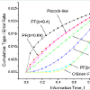
Commonly used classes of error-spending functions are O’Brien-Fleming-like spending function, the Pocock-like function, and the power-function family. The power-function family, π(I) =αtb is valuable as it, can approximate the others error-spending functions well (Figure 1).
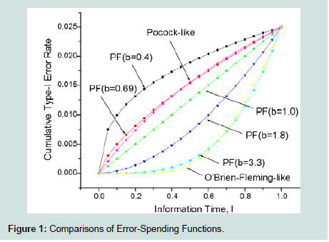
Figure 1 : Comparisons of Error-Spending Functions.
Sample-Size Re-estimation Design
A sample-size reestimation (SSR) design refers to an adaptive design that allows for sample-size adjustment or re-estimation based on the review of interim analysis results. The sample-size requirement for a trial is sensitive to the treatment effect and its variability. An inaccurate estimation of the effect size or its variability could lead to an underpowered or overpowered design, neither of which is desirable. If a trial is underpowered, it will not be able to detect a clinically meaningful difference, and consequently could prevent a potentially effective drug from being delivered to patients. On the other hand, if a trial is overpowered, it could lead to unnecessary exposure of many patients to a potentially harmful compound when the drug, in fact, is not effective. In practice, it is often difficult to estimate the effect size and variability because of many uncertainties during protocol development. Thus, it is desirable to have the flexibility to re-estimate the sample-size in the middle of the trial.There are two types of sample-size reestimation procedures, namely, sample-size reestimation based on blinded data and samplesize reestimation based on unblinded data. In the first scenario, the sample adjustment is based on the (observed) pooled variance at the interim analysis to recalculate the required sample-size, which does not require unblinding the data. In this scenario, the Type-I error adjustment is practically negligible; in fact, FDA and other regulatory agencies typically regard this type of sample size adjustment to be unbiased and without any statistical penalty. In the second scenario, both the effect size and its variability are re-assessed, and sample-size is adjusted based on the updated information. The statistical method for adjustment could be based on the observed effect size or the calculated conditional power.
The main statistical challenge of SSR compared to GSD is that unlike in GSD, in which the √I1z1 and √I1z2 in the test statistic T2 are independent, in SSR, because √I1z2 is a function of the second stage sample size n₂ that depends on the observed treatment difference or z₁ from the first stage data. The joint distribution of T1 and T2 is much more complicated than in GSD. Several solutions have been roposed, including the fixed weight method [30], the method of adjusting stopping boundary through simulations [44,56], and promising-zone methods [31,32].
The fixed weight method for combining test statistics usually takes the square-root of the information time at the interim analysis with the original final sample size N0 as the denominator, i.e., 
T2=√I0z1+√1-I0z2
The weighted Z-statistic approach (7) is flexible in that the decision to increase the sample size and the magnitude of sample size increment are not mandated by pre-specified rules. Chen, DeMets, and Lan proposed the Promising-Zone method, where the unblinded interim result is considered “promising” and eligible for SSR if the conditional power is greater than 50 percent, equivalently, the sample size increment needed to achieve a desired power does not exceed a prespecified upper bound [31]. The Promising-Zone method may be justifiable to effectively put resources on drug candidates that are likely effective or that might fail only marginally at the final analysis with the original sample size, based on the information seen at the interim analysis.
Some researchers prefer using an equal weight for each patient, i.e., “one patient, one vote”. The “one patient, one vote” policy for the test statistic at the second stage does not follow the above formulation because the patients from the first stage (T1) have potentially two opportunities to vote in the decision-making (rejecting or not rejecting the H0), one at the interim analysis and the other at the final analysis, while patients from the second stage have at most one time to vote when the trial continues to the second stage.
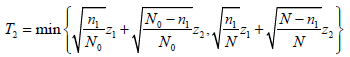
Chen, DeMets, and Lan proposed a variation of the Promising-Zone method, using a conservative test statistic for the second stage [31]:
where z1 and z2 are the usual Z-statistic based on the subsamples from stages 1 and 2, respectively. n₁ is the sample size at the interim analysis, N0 is the original final sample size and N is the new final sample size after adjustment based on the interim analysis.
Using this modified test statistic, the authors proved that when the conditional probability based original sample size is larger than 50%, then adjusted sample size, i.e., increasing the sample size when the unblinded interim result is promising will not inflate the type I error rate and therefore no statistical adjustment is necessary.
Mehta and Pocock proposed another Promising-Zone method, in which they define the promising zone as the interim p-value p1 between 0.1587 (z1=1.206) and 0.0213 (z1=2.027) [32]. They chose these values because when one-sided p-value p1 is larger but close to 0.1 at the interim analysis with information time Τ=0.5, the trial is likely to marginally fail to reject H0 at the final analysis with p-value around 0.06 to 0.15. Those drug candidates are likely clinically effective, thus we want to “save” those trials and allow them a better chance to show statistical significance by increasing the sample size. If the p1 is, say, larger than 0.2 (0.4 for two-sided p-value), we will stop the trial earlier at the first stage. For practical purposes, we recommend the following approach: combine the futility boundary with the upper bound of the promising zone and recommend using β1 =0.2 for the one-sided p-value at the interim analysis with information time 0.5.
Current SSR methods [30], down weighting patients from the second stage, are not very efficient. Tsiatis and Mehta argue that GSD is more efficient than SSR design [33]. On the other hand, GSD is just a special case of SSR design and “the part” cannot be larger than “the whole”. More efficient SSR designs are desirable and need more research.
Pick-Winner Design
The multiple-arm dose response study has been studied since the early 1990s. Under the assumption of monotonicity in dose response, Williams proposed a test to determine the lowest dose level at which there is evidence for a difference from the control [91]. Cochran, Amitage, and Nam developed the Cochran-Amitage test for monotonic trend. For the strong familywise Type-I error control, Dunnett’s test and Dunnett & Tamhane based on the multivariate normal distribution is most often used and Rom, Costello, Connell proposed a closed set test procedure [92-98]. A recent addition to the adaptive design arsenal is multiple-arm adaptive designs. A typical multiple-arm confirmatory adaptive design (variously called dropthe-loser, drop-arm, pick-the-winner, adaptive dose-finding design, or Phase II/III seamless design) consists of two stages: a selection stage and a confirmation stage. For the selection stage, a randomized parallel design with several doses and a placebo group is employed. After the best dose (the winner) is chosen based on numerically “better” observed responses, the patients of the selected dose group and placebo group continue to enter the confirmation stage. New atients are recruited and randomized to receive the selected dose or placebo. The final analysis is performed with the cumulative data of atients from both stages [44,99].Recent additions to the literature include Bretz et al. who studied confirmatory seamless Phase II/III clinical trials with hypothesis selection at interim. Huang, Liu, and Hsiao proposed a seamless design to allow pre-specifying probabilities of rejecting the drug at each stage to improve the efficiency of the trial [100,101]. Posch, Maurer, and Bretz described two approaches to control the Type I error rate in adaptive designs with sample size reassessment and/or treatment selection [102]. The first method adjusts the critical value using a simulation-based approach that incorporates the number of patients at an interim analysis, the true response rates, the treatment selection rule, etc. The second method is an adaptive Bonferroni-Holm test procedure based on conditional error rates of the individual treatment-control comparisons. They showed that this procedure controls the Type I error rate, even if a deviation from a pre-planned adaptation rule or the time point of such a decision is necessary. Shun, Lan and Soo considered a study starting with two treatment groups and a control group with a planned interim analysis [26]. The inferior treatment group will be dropped after the interim analysis. Such an interim analysis can be based on the clinical endpoint or a biomarker. The unconditional distribution of the final test statistic from the ‘winner’ treatment is skewed and requires numerical integration or simulations for the calculation. To avoid complex computations, they proposed a normal approximation approach to calculate the Type-I error, the power, the point estimate, and the confidence intervals. Heritier, Lo and Morgan studied the Type-I error control of seamless unbalanced designs, issues of noninferiority comparison, multiplicity of secondary endpoints, and covariance adjusted analyses [103]. Further extensions of seamless designs that allow adaptive designs to continue seamlessly either in a subpopulation of patients or in the whole population on the basis of data obtained from the first stage f a Phase II/III design have also been developed. Jenkins, Stone, and Jennison proposed design adds extra flexibility by also allowing the trial to continue in all patients but with both the subgroup and the full population as coprimary populations when the Phase II and III endpoints are different but correlated time-to-event endpoints [104].
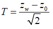
Shun, Lan and Soo found that under the global null hypothesis, common z statistic Zw from the winner group is approximately normal distributed with mean 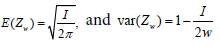 [26]. Therefore, they proposed a the test statistic
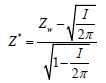
[26]. Therefore, they proposed a the test statisticwhich has approximately the standard normal distribution.
The approximate p-value can be easily obtained: pA=1-Φ (Z*).
The exact p-value, based on the exact distribution of Zw, is given byp =pA+ 0.0003130571(4.444461T) - 0.00033.
For a general K-group trial, we define the global null hypothesis as HG: μ0 = μ1 = μ2...μk and the hypothesis tesm (winner) and the control as
H0: μ0 = μw, w = winner (selected arm)
Under larger sample size assumptions, given the observed valuesxi and standard deviation in group i (i=0 and w),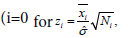 placebo and w for the winner) has a standard normal distribution. The test statistic for the comparison between the placebo group and the winner group can be defined as
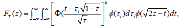
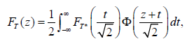
Chang and Chang and Wang prove that the distribution of T under HG is given by
where the standard normal distribution pdf and cdf, annotated by φ and Φ, respectively [27,56].
If the purpose of the interim analysis is only for picking the winner, the stopping boundary cα can be determined using FT (cα ) =1-α for a one-sided significance level α. Numerical integration or simulation can be used to determine the stopping boundary and power. For Τ=0.5, the numerical integrations give cα=2.352, 2.408, 2.451, and 2.487 for K=4, 5, 6, and 7, respectively. The power of winner designs can be easily obtained from simulations.
Pick-winner design can improve the trial efficiency, but how to set the selection criteria for winner to optimize the adaptive trial is still unclear and requires further investigation.
Add-Arm Design
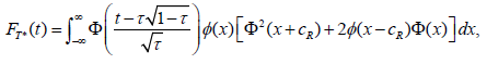
In a winner design, patients are randomized into to all arms (doses) and at the interim analysis, inferior arms will be dropped. Compared to traditional dose-finding design, this adaptive design can reduce the sample size by not carrying over all doses to the end of the trial or dropping the losers earlier. However, it does require all the doses have to be explored. For unimodal response curves, Chang, Chang and Wang propose an effective adaptive dose-finding design that allows adding arms at interim analysis [27,56]. The trial design starts with two arms and depending on the response of the two arms and the unimodality assumption, we can decide which new arms to be added. This design does not require exploration of all arms (doses) to find the best responsive dose, therefore may further reduce the sample size from the dropping-loser design by as much as 20%.Under the HG, the cdf of the test statistic T, formulated from the placebo and the finally selected arm is given by
where cdf FT* is given by
If we examine the design that only allows us to reject HG at the final analysis for the moment: if the T≥cα, test we would reject H0. In such a case, the stopping boundary can be determined using TF (cα) for an one-sided significance level α. Numerical integration or simulation can be used to determine the stopping boundary and power. For example, the simulation shows rejection boundary to be cα=2.267 for a one-sided α=0.025.
Under unimodal response, Chang-Wang’s three-stage add-arm design is usually more powerful that the 2-stage drop-arm design primarily because the former takes the advantage of the knowledge of unimodility of response. If the response is not unimodal, we can use that prior knowledge to rearrange the dose sequence so that it becomes unimodal response.
In an add-arm design, all arms are usually selected with equal chance when all arms have the same expected response, but the probability of rejection is different even when all arms are equally effective [27]. This feature allows us to effectively use the prior information to place more effective treatments in the middle but at the same time the two arms in the first stage have a large enough separation in terms of response to increase the power.
In an add-arm design, dose levels don’t have to be equally placed or based on the dose amount. The arms can be virtual dose levels or combinations of different drugs. Furthermore, the number of arms and the actual dose levels do not have to be prespecified, it can be decided after the interim analyses.
An add-arm design can further reduce the sample size from a pick-winner design, but it adds a complexity to the trial: there are three stages in an add-arm design, but two stages in a pick-winner design. On one hand, reducing sample size will reduce the time for the trial. On the other hand, a staggered patient enrollment in three stages will take longer than to enroll patients than with two stages.
Adaptive Randomization Design
Response-adaptive randomization or allocation is a randomization technique in which the allocation of patients to treatment groups is based on the responses (outcomes) of the previous patients. The main purpose is to provide a better chance of randomizing the patients to a superior treatment group based on the knowledge about the treatment effect at the time of randomization. As a result, responseadaptive randomization takes ethical concerns into consideration.In the response-adaptive randomization, the response does not have to be on the primary endpoint of the trial; instead, the randomization can be based the response on a biomarker. Scholars including Zelen, Wei and Durham, Wei, et al., Stallard and Rosenberger, Hu and Rosenberger, and many others have contributed in this area [19,105-108].
Fiore et al. use a response-adaptive randomization based on Bayesian posterior distribution of treatment effect given the observed response data and discuss the application is a point-of-care clinical trial with insulin administration [109]. Fava et al., Walsh et al. and Doros, et al. studied two-stage re-randomization adaptive designs and analyses in trials with high placebo effect [110-112].
The well-known response-adaptive models include the playthe-winner (PW) model and the randomized play-the-winner (RPW) model. A RPW model is a simple probabilistic model used to sequentially randomize subjects in a clinical trial [106,113]. The RPW model is useful for clinical trials comparing two treatments with binary outcomes. In the RPW model, it is assumed that the previous subject’s outcome will be available before the next patient is randomized. At the start of the clinical trial, an urn contains a0 balls representing treatment A and b0 balls representing treatment B, where a0 and b0 are positive integers. We denote these balls as either type A or type B balls. When a subject is recruited, a ball is drawn and replaced. If it is a type A ball, the subject receives treatment A; if it is a type B ball, the subject receives treatment B. When a subject’s outcome is available, the urn is updated as follows: A success on treatment A (B) or a failure on treatment B (A) will generate an additional a1 (b1) type-B balls in the urn. In this way, the urn builds up more balls representing the more successful treatment.
RPW can reduce the number of subjects assigned to the inferior arm, however, for Phase three trials, imbalanced randomization can reduce the power [44,114]. In small studies, response-adaptive randomization can be more problematic in causing potential confounders imbalance than a classical design. Ning and Huang proposed response-adaptive randomization with adjustment for covariate imbalance [115]. There are also several optimal RPW designs have been proposed based on proportion difference, odd ratio, and relative risk [116]. However, optimal RPW designs in terms of power require further development.
Adaptive Dose-Escalation Design
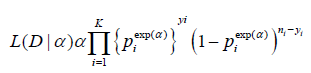
Adaptive Dose-escalation design is a type of adaptive designs that is not based on Type-I error control and it is often used for earlyphase studies. Dose-escalation is often considered in early phases of clinical development for identifying maximum tolerated dose (MTD), which is often considered the optimal dose for later phases of clinical development. An adaptive dose-finding (or dose-escalation) design is a design at which the dose level used to treat the next-entered patient is dependent on the toxicity of the previous patients, based on some traditional escalation rules. Many early dose-escalation rules are adaptive, but the adaptation algorithm is somewhat ad hoc. Recently more advanced dose-escalation rules have been developed using modeling approaches (frequentist or Bayesian framework) such as the continual reassessment method (CRM) [1,22] and other accelerated escalation algorithms. These algorithms can reduce the sample-size and overall toxicity in a trial and improve the accuracy and precision of the estimation of the MTD.The CRM is often presented in an alternative forms [24]. In practice, we are usually prespecify the doses of interest, instead of any dose. Let (d1,...,dk) be a set of dose and (p1,...,pk) be the corresponding prespecified probability, called the “skeleton”, satisfying p1<p2,...<pk. The dose-toxicity model of the CRM is assumed to be
Pr (toxicity at di)=πi(α)=Piexp(α),i=1,2,...,K,
where α is an unknown parameter. Parabolic tangent or logistic structures can also be used to model the dose-toxicity curve.
Let D be the observed data: yi out of ni patients treated at dose level i have experienced the dose-limiting toxicity (DLT). Based on the binomial distribution, the likelihood function is
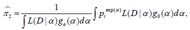
Using Bayes’ theorem, the posterior means of the toxicity probabilities at dose j can be computed by
where g0 (α) is a prior distribution for α, for example, α∼N(0,σ2).
Ivanova and Kim study dose-finding for binary ordinal and continuous outcomes with monotone objective function or utility function [23]. Ivanova, Flournoy, Chung proposed a method for cumulative cohort design for dose-finding. Lee and Cheung proposed a model calibration in the continual reassessment method [117,118]. CRM designs with efficacy-safety trade-offs are studied by Thall and Cook, Yin, Li, and Ji, and Zhang, Sargent, and Mandrekar [119-122]. Bayesian adaptive designs with two agents in Phase-I oncology trial are studied by Thall, et al., Yin and Yuan [123-125]. Bayesian adaptive designs for different phases of clinical trials are covered in the book by Berry, Carlin, Lee, Muller [76].
CRM is relatively monitor-intensive adaptive design since it is requires calculation to determine the next patients assignment based on the real-time data. When there is a delayed response, the efficiency of the design will be largely lost. There also rules to prevent too fast dose-jump to protect patient’s safety in the trial, which also further reduce the efficiency CRM designs.
Randomized Concentration-Controlled Trial
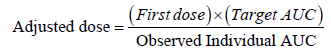
Sanathanan and Peck published a simulation study where they investigated the improvement in sample size and efficiency that can be gained from the randomized concentration-controlled trial (RCCT) design [28]. An RCCT can be considered “individualized treatment” or “personalized medicine” because, for each patient, dosage is adjusted according to the targeted concentration. Such dose modification or adaptation is based on the observed plasma concentration of the previous doses. The idea is that since the randomization point is moved closer to the clinical endpoint in the chain of causal events, randomizing patients to the defined target concentrations, as opposed to doses, makes it possible to reduce the within-group variability in the response variable in relation to the randomization variable [126]. The statistical methods for the dosage prediction and adjustments (so-called adaptive feedback strategy) can be based on the simple dose-proportionality assumption (AUC is proportional to the dose) or to the maximization of the Bayesian posterior probability of achieving the target concentration. Research showed that RCCT has the following advantages: (1) power will increase or sample size will reduce, (2) study power will be less sensitive to high variability in PK, (3) less confounded estimation of exposure-response, and (4) increased safety with narrow therapeutic window drugs [28,29,127]. The idea of RCCT can also be used for adjusting doses for each patient based on the target biomarker or PD response. Such a trial is called randomized biomarker-controlled trial (RBCT).Since pharmacological effects are driven by the concentration at the site of action, the systemic drug concentrations are clearly in the causal pathway of drug action. Biomarkers and PD responses, on the other hand, may or may not be in the causal pathway, and thus can be very misleading markers when they are not (e.g. when the biomarker reflects an off-target effect). Moreover, it is well known that many biomarkers and PD responses are inherently more variable than drug concentration measurements. Thus, there is no “conceptual” advantage of the RBCT over the RCCT --- blind employment of the RBCT can even lead to greater inefficiency than that of the RCT design. Note that both RCCT and RBCT trial outcomes present statistical inferential challenges when the frequentist approach is employed to assess dose-response, since dose assignment is not randomized in either design.
Some common algorithms for adjusting dosage are:
(1) Adjustment based dose proportionality (Cella, Danhof, andPasqua, 2012):
(2) Adjustment based on linearity on log-scale (Power model):
LogC = β0+β1log d+ ε,
where d is dose and ε is the within subject variability.
The parameters β0 and β1 can be frequentist or Bayesian posterior estimates. After the expected (average) value of dose d to achieve the target concentration C can be determined.
Biomarker-Adaptive Design
Biomarker-adaptive design (BAD) refers to a design that allows for adaptations using information obtained from biomarkers. A biomarker is a characteristic that is objectively measured and evaluated as an indicator of normal biologic or pathogenic processes or pharmacologic response to a therapeutic intervention [128]. A biomarker can be a classifier, prognostic, or predictive marker.A classifier biomarker is a marker that usually does not change over the course of the study, like DNA markers. Classifier biomarkers can be used to select the most appropriate target population, or even for personalized treatment. Classifier markers can also be used in other situations. For example, it is often the case that a pharmaceutical company has to make a decision whether to target a very selective population for whom the test drug likely works well or to target a broader population for whom the test drug is less likely to work well. However, the size of the selective population may be too small to justify the overall benefit to the patient population. In this case, a BAD may be used, where the biomarker response at interim analysis can be used to determine which target populations should be focused on.
A prognostic biomarker informs the clinical outcomes, independent of treatment. They provide information about the natural course of the disease in individuals who have or have not received the treatment under study. Prognostic markers can be used to separate good- and poor-prognosis patients at the time of diagnosis. If expression of the marker clearly separates patients with an excellent prognosis from those with a poor prognosis, then the marker can be used to aid the decision about how aggressive the therapy needs to be.
A predictive biomarker informs the treatment effect on the clinical endpoint. Compared to a gold-standard endpoint, such as survival, a biomarker can often be measured earlier, easier, and more frequently. A biomarker is less subject to competing risks and less affected by other treatment modalities, which may reduce samplesize. A biomarker could lead to faster decision-making. In a BAD, “softly” validated biomarkers are used at the interim analysis to assist in decision-making, while the final decision can still be based on a gold-standard endpoint, such as survival, to preserve the Type-I error [56].
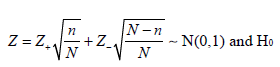
We briefly discuss the population enrichment design. Denote the treatment difference between the test and control groups by δ+, δ-, and δ, for biomarker-positive, biomarker-negative, and overall patient populations, respectively. The test statistics for the treatment effects in biomarker-positive, biomarker-negative, and the overall patient populations are denoted by Z+, Z-, and Z, respectively.
The test statistic for overall population is
where n and N are the sample size for the biomarker-positive patients and overall patients in the trial, the correlation coefficient between Z and Z+ is
For adaptive designs, the information of Z-, Z+, and Z can be used to determine/change the randomization - biomarker enrichment design [37]. Wang studied the utility of predictive biomarker in adaptive design and discovered that the correlation coefficient ρ between the biomarker and primary endpoint in a clinical trial is not necessarily the main predicting factor [48]. For this reason, Wang and Chang developed a two-level hierarchical model, called biomarker informed adaptive design [50]. Wang, Chang, and Sandeep developed a biomarker-informed add-arm design for unimodal response [49].
The main challenges in utilization of biomarkers in clinical trials with classical or adaptive design are (1) usually a small set of data available with great uncertainties, and (2) there are often set of markers, not single marker, that affect the outcomes of the primary endpoint, which will make the model more complicated and require more data points or subjects to produce a valid model.
Clinical Trial Simulation
Due to the complexity of adaptive trials, extensive simulations are often required during the design and conduct of clinical trials, and even in the analysis of trial data, simulation can be used to evaluate the robustness of the results.Clinical trial simulation (CTS), also called Monte Carlo Similation, is a process that mimics clinical trials using computer programs. CTS is particularly important in adaptive designs for several reasons: (1) the statistical theory of adaptive design is complicated with limited analytical solutions available under certain assumptions; (2) the concept of CTS is very intuitive and easy to implement; (3) CTS can be used to model very complicated situations with minimum assumptions, and Type-I error can be strongly controlled; (4) using CTS, we can not only calculate the power of an adaptive design, but we can also generate many other important operating characteristics such as expected sample-size, conditional power, and repeated confidence interval - ultimately this leads to the selection of an optimal trial design or clinical development plan; (5) CTS can be used to study the validity and robustness of an adaptive design in different hypothetical clinical settings, or with protocol deviations; (6) CTS can be used to monitor trials, project outcomes, anticipate problems, and suggest remedies before it is too late to make modifications; (7) CTS can be used to visualize the dynamic trial process from patient recruitment, drug distribution, treatment administration, and pharmacokinetic processes to biomarkers and clinical responses; and finally, (8) CTS has minimal cost associated with it and can be done in a short time.
In protocol design, simulations are used to select the most appropriate trial design with all necessary scenarios considered. In trial monitoring, simulations are often used to guide the a necessary adaptations, such as stop or continue the trial, sample-size adjustment, evaluation of conditional power or probability of success given the interim observed data, shift of patient randomization probability, change of target patient population, etc. In the analysis of trial data, CTS can be used for evaluation of missing data impact and effect of other factors to evaluate the internal validity and external validity of the conclusions.
Chang provide comprehensive CTS techniques in classical and adaptive designs using SAS and he also provide introductory to adaptive design using R [53,56]. For broad coverage of Monte Carlo simulations in the pharmaceutical industry, we recommend the text “Monte Carlo Simulations in the Pharmaceutical Industry” by Chang [129]. The scope covered in the 13 chapters includes: (1) Meta-simulation in pharmaceutical industry game, (2) macrosimulation in pharmaceutical R & D, (3) Clinical Trial Simulation, (4) simulation in clinical trial management and execution, (5) simulation for prescription drug commercialization, Molecular design and simulation, (6) Disease modeling and biological pathway simulation, (7) Pharmacokinetic simulation, (8) Pharmacodynamic simulation, (9) Monte Carlo for inference and beyond, and others.
A recent book edited by Menon and Zink covers a range ofadaptive design simulation using SAS. Many adaptive design practicians have contributed to the books. It is a good reference in adaptive trial designs [130].
Deciding Which Adaptive Design to Use
When we design our first adaptive trial, we will need to know how to start and we may even wonder if the adaptive design would really be better than a classic design. What if we miss something or something goes wrong?The first step is to choose an appropriate type of adaptive design based on the trial objective(s). If it is a Phase III confirmatory trial, we may consider group sequential design or SSR design. If the timing of the analyses or the number of analyses are expected to change for practical reasons (e.g., the availability of DMC committee members or safety concern requires more interim analyses), we should choose GSD with error-spending approach. If the estimation of effect size is very unreliable, we should use SSR. If the number of doses (arms) to be considered is more than two (include the control arm) and, for example, we don’t know exactly which dose (treatment regimens or drug combinations of drugs) is the best (or good enough), we should use a winner or add-arm design. Note that an add-arm design is usually statistically more efficient than a drop-arm design, but also adds a little more to the complexity of the trial design and conduct. If a screening test of a stable biomarker is available (and practical) and we expect the test drug may have different efficacy and/or safety profiles for patients with and without the biomarker, we can use a biomarker enrichment design, in which the interim analysis will be used for deciding which population should be the target. If the biomarker is expected to respond to the drug and it can be measured earlier at the interim analysis than the primary endpoint of the trial, then we can use a biomarker-informed adaptive design. The response-adaptive design can be based on the primary endpoint or the biomarker response if the former is not available at the time of randomization.
In any setting, we should perform the clinical trial simulations to further evaluate and compare the operating characteristics of different designs or designs with different parameters. If the trial is an early stage design for a progressive disease such as cancer, we can use dose-escalation design in which the dose gradually increases to protect the patients’ safety. The next step is to determine whether a superiority, non-inferiority, or equivalence trial is needed based on the primary trial objective and the regulatory requirement and to determine the number of analyses points. The timing and number of interim analysis will be dependent on the safety requirement (some need more frequent safety monitoring), statistical efficiency (more interim analyses might reduce the sample size, need CTS to check), and practicality (complexity of the trial conduct and associated time and cost). We may need to consider some special issues, such as paired data or missing data, or other parameters. We would again conduct broad simulations with various design features/parameters and choose the most appropriate one based on proposed evaluation matrix. Finally, we need to consider the practical issues: How long will the trial take? Should we halt the trial when we performed the interim analysis? How fast can we do the interim analysis including the data cleaning. Will the recruitment speed and delayed response jeopardize the adaptive design? Who will perform the interim analysis and write the interim monitoring plan or DMC Charter? Dose the regulatory agency agree on the non-inferiority margin if a noninferiority adaptive trial? How the randomization be done? Can IVRS (interactive voice response system) support the adaptive design? How will the drug be distributed to the clinic sites? How will the primary analysis for the adaptive trial data be done?
Determining design parameters
The trial objectives are generally determined by the study team at a pharmaceutical company. The prioritization of the objectives is usually based on the clinical and commercial objectives and the trial design is optimized to increase the likelihood of success.After the objectives are determined, we choose the primary endpoint (a normal, binary, survival endpoint, etc.) to best measure the objectives and the timing of when the endpoints should be measured, and decide whether it is based on the change from baseline or the raw measure at a post-baseline time point. Next, we estimate the expected value for the endpoint in each treatment group based on prior information, which might be an early clinical trial, a preclinical study, and/or a published clinical trial results by other companies for the same class drug. The reliability of the historical data will affect our choice of the adaptive design.For Phase III trials, the Type-I error rate must typically be controlled at one-sided significance level α=0.025 for most of drugs. For early phase trials, α can be more flexible. A smaller α will reduce the false positive drug candidate entering late phase trials, but the same time increase the chance of eliminating the effective drug candidates from further studies, unless we increase the sample size to keep the Type-II error rate β unchanged.The most important factors (operation characteristics) for selecting a design with interim analyses are the expected sample size and maximum sample size for a fixed power [56]. If we wish to reduce the expected cost, we might want to choose a design with minimum expected sample size; if we wish to reduce the maximum possible cost, we might want to consider a design with minimum total sample size. In any case, we should carefully compare all the stopping probabilities between different designs before determining an appropriate design. O‘Brien-Fleming’s boundary is very conservative in early rejecting the null hypothesis. Pocock boundary applies a constant boundary on p-scale across different stages [131]. To increase the probability of accepting the null hypothesis at earlier stages, a futility boundary can be used. In general, if we expect the effect size of the treatment is less than what we have assumed and the cost is your main concern, we should use an aggressive futility boundary to give a larger stopping probability at the interim in case the drug is ineffective or less effective. On the other hand if we worry about the effect size might be under-estimated, we should design trial with aggressive efficacy stopping boundary (Pocock-like rather than O‘Brian-Fleming-like) to boost the probability early efficacy stopping in case the drug is very effective.
Evaluation matrix of adaptive design
To choose an adaptive design among several options, we have to consider the trial objective, the cost, the duration of the study, the recruitment challenges, execution challenges, how to get the team and the regulatory authority buy-in. We can consider the impact of failure and success of the trial using a utility function [56]:U = ∫ R(θ)w(R)f(θ)dθwhere θ is the design input parameter vector, R is outcome or result vector component or operating characteristics, w is the corresponding weight function w(R), measuring the relative importance of R among all possible Rs, and f(θ) is the prior distribution of θ.Practically, we may select three or more typical scenarios for the main evaluation: H0, Hs, and Ha. Their weighted average N, the maximum sample size Nmax, number of analyses, power, utility, safety management, complexity of the trial design and conduct can compose the evaluation matrix and it is convenient to summarized in a Table like (Table 1).
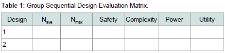
Table 1 : Group Sequential Design Evaluation Matrix.
Controversies and Challenges
Equal weight principleThere are criticisms about the “unequal weights” in sample size reestimation with the fixed weight approach. However, even in the group sequential design without sample size reestimation, the “one person one vote” principle is violated because earlier enrolled patients have more chances to vote in the decision-making (rejecting or accepting the null hypothesis) than later enrolled patients. In twostage group sequential design, the first patient has two chances to “vote”, at the interim and final analyses, while the last patient has only one chance to vote at the final analysis. The impact of each individual vote is heavily dependent on the alpha spent on each analysis, i.e., the stopping boundaries.
From an ethical point of view, should there be equal weight for everyone, one vote for one person? Should efficacy be measured by the reduction in number of deaths or by survival time gained? Should it be measured by mean change or percent change from baseline? All these scenarios apply a different “equal weight” system to the sample. Suppose you have a small amount of a magic drug, enough to save only one person in a dying family: the grandfather, the young man, or the little boy. What should you do? If you believe life is equally important for everyone regardless of age, you may randomly (with equal probability) select a person from the family and give his/her the drug. If you believe the amount of survival time saved is important (i.e., one year of prolonged survival is equally important to everyone), then you may give the drug to the little boy because his life expectancy would be the longest among the three family members. If you believe that the impact of a death on society is most important, then you may want to save the young man, because his death would probably have the most negative impact on society. If these different philosophies or beliefs are applied to clinical trials, they will lead to different endpoints and different test statistics with different weights. Even more interesting, statisticians can optimize weights to increase power of a hypothesis test.
Biasedness
In statistics, the bias of an estimator is the difference between this estimator’s expected value and the true value of the parameter being estimated. If there is no difference, the estimator is unbiased. Otherwise the estimator is biased. Thus the term, bias, in statistics is an objective statement about a random function, different from commonly used English “bias”. Bias can also be measured with respect to the median, rather than the mean (expected value), in which case one distinguishes median-unbiased from the usual meanunbiasedness property.
An estimate is most time different from the truth, but that does not make the estimator or the estimation method bias. If an estimation method (estimator) of the treatment effect is the same average value as the true treatment effect under repeated experiments, the estimator or method is unbiased for estimating that parameter (i.e., treatment effect).
Bias has usually nothing to do the sample size, though a smaller sample size usually gives a less precise estimate. When an estimator is approaching the truth of the parameter as the sample size goes to infinity, we call the estimator is “consistent”. In adaptive design bias can be defined differently under repeated experiments: conditional on the stage when the trial stops or unconditionally average over the all estimates regardless when the trial stops. From Bayesian’s perspective, the statistical biasedness is not a concern. One of the arguments is that the same experiment naiver repeats.
Why is the naive or maximum likelihood estimate biased in an adaptive trial? To use a simple example to illustrate, if in a GSD trial with possible early efficacy stopping, then data that are extreme positive will be excluded from the final analysis because the extreme positive results will lead to early stopping of the trial. The result is a downward bias of MLE estimate of the treatment effect.
If we view from the pharmaceutical company’s perspective, we can see all the trial results whether is positive or negative, but patients only see the positive results of marketed drugs, which include the true positive or false positive. What the FDA and regulatory agencies see is somewhere in between. If we average what people can see, then patients and FDA have biased views on treatment effect, statistically.
Conditional Biasedness and correction has be studied by Jennison and Turnbull, Pickard and Chang, Luo, Wu and Xiong, Sampson and Sill, Stallard, Todd, Whitehead, Tappin, Liu et al., Tsiatis, Rosner, & Mehta, and Whitehead among others [66,71,74,132-138].
Type-I error control and multiplicity
The controversies surrounding the Type-I error control and multiplicity of hypothesis testing will never be completely resolved, even though there are major advancement in methodology [139-141]. Here we are going to discuss the controversies particular to adaptive designs.
Patient-Statistician Paradox: Suppose new compounds A and B for cancer treatment were tested in the same clinical trial with a common control [57,58,139]. For drug A, only one analysis was performed at the final analysis with 500 patients treated in drug A and 500 patients in control; the null hypothesis was rejected and drug is claimed to be efficacious. For drug B, a GSD is used with 10 analyses performed at each 50-patient increment, at each analysis 10% α were spent, and unfortunately, every time the rejection H0 was just missed. Therefore, drug B is not efficacious based on statistical hypothesis testing. At the final analysis, however, the observed median survival time was two years for drug B and only 6 months for drug A. The question is: a patient who is a statistician would take drug A or B? On one hand, as a statistician he may believe importance of Type-I error control and determine not to take drug B. On the other hand, as a patient he really wants to survive two year rather than six months! It is not based on one’s intuition, but one can justify it by saying: “The chemical structure of the drug will not change just because statistical method changes, thus the interim analyses should not affect one’s choice of the drug”.
Here, we can see two different concepts of the effectiveness of a drug. One is the physical properties of the test compound, which will not change as the hypothesis test procedure changes (e.g., one test versus multiple tests). The other is the statistical property that will change since it reflects an aggregated attribute of a group of similar things - the similarity principle of sciences [58].
At the moment, for early phase trials, Type-I error control is not strictly enforced, Bayesian methods can also be used in those trials [1,20,25,76,140]. CRM we discussed earlier is a typical Bayesian adaptive design for earlier clinical trials. Personalized medicine is the future for the patients, however, to be able to effectively develop personalized medicine, adaptive design can be a great tool [142,143].
Practical challenges
There are challenges associated with adaptive design. Statistical methods are available for most common adaptive designs, but for more complicated adaptive designs, the methodologies are still in development.
Operationally, an adaptive design often requires real-time or near real-time data collection and analysis. In this regard, data standardizations, such as Clinical Data Interchange Standards Consortium (CDISC) and Electronic Data Capture (EDC), are very helpful in data cleaning and reconciliation. Note that not all adaptive designs require perfectly clean data at interim analysis, but the cleaner the data are, the more efficient the design is. Adaptive designs require the ability to rapidly integrate knowledge and experiences from different disciplines into the decision-making process and hence require a shift to a more collaborative working environment among disciplines.
From a regulatory standpoint, there is a draft (not for implementation) FDA’s guidance for adaptive designs at the moment. Adaptive trials are reviewed on a case-by-case basis. Naturally there are fears that a protocol using this innovative approach may be rejected, causing a delay.
The initial fear that the interim unblinding may potentially cause bias and put the integrity of the trial at risk is still there, but, level of anxiety is reduced as the knowledge and experiences of Adaptive design are accumulating. Therefore, the unblinding procedure should be well established before the trial starts, and frequent unblinding should be avoided. Also, unblinding the premature results to the public could jeopardize the trial.
Summary
Adaptive designs can reduce time and cost, minimize toxicity, and help select the best dose for the patients and improve selection of the target populations. With adaptive design, we can develop better science for testing new drugs, and in turn, better science for prescribing them. Adaptive design will promote the personalized medicine to get the right drug to the right patient with right amount at the right time.Adaptive design may require fewer patients, less trial material, sometimes fewer lab tests, less work for data collection and fewer data queries to be resolved. Adaptive design is a sequential datadriven approach. It is a dynamic process that allows for real-time learning. It is flexible and allows for modifications to the trial, which make the design cost-efficient and robust against the failure. Adaptive design is a systematic way to design different phases of trials, thus streamlining and optimizing the drug development process. In contrast, the traditional approach is composed of weakly connected phase wise processes. Adaptive design is a decision-oriented, sequential learning process that requires up-front planning and a great deal of collaboration among the different parties involved in the drug development process. To this end, Bayesian methodology and computer simulation play important roles. Finally, the flexibility of adaptive design does not compromise the validity and integrity of the trial or the development process.
Adaptive design methods represent new territory in drug development, representing a revolution in pharmaceutical research and development. Using adaptive designs, we can increase the chances for success of a trial with a reduced cost. Bayesian approaches provide a powerful tool for optimizing trial designs and clinical development plans. Clinical trial simulations offer a powerful tool to design and monitor trials.
This innovative approach requires careful upfront planning and the ability to rapidly integrate knowledge and experiences from different disciplines into the decision-making process, require a shift to a more collaborative working environment among disciplines.
Acknowledgements
Many thanks to Dr. Robin Bliss for her careful review and numerous corrections and suggestions. Thanks to the two anonymous reviewers for their constructive comments. Their comments have greatly improved the manuscript.References
- Chang M, Chow SC (2005) A hybrid Bayesian adaptive design for dose response trials. J Biopharm Stat 15: 667-691.
- Gallo P, Chuang-Stein C, Dragalin V, Gaydos B, Krams M, et al. (2006) Adaptive designs in clinical drug development--an executive summary of the PhRMA working group. J Biopharm Stat 16: 275-283.
- Dragalin V (2006) Adaptive designs: terminology and classification. Drug Inf J 40: 425-435.
- Bauer P (1989) Multistage testing with adaptive designs (with Discussion). Biometrie und Informatik in Medizin und Biologie 20: 130-148.
- Bauer P, Kohne K (1994) Evaluation of experiments with adaptive interim analysis. Biometrics 50: 1029-1041.
- Bauer P, Kohne K (1996) Evaluation of experiments with adaptive interim analyses. Biometrics 52: 380.
- Bauer P, Rohmel J (1995) An adaptive method for establishing a doseresponse relationship. Stat Med 14: 1595-1607.
- Bauer P, Bretz F, Dragalin V, Koniga F, Wassmere G (2016) Twenty-five years of confirmatory adaptive designs: opportunities and pitfalls. Stat Med 35: 325-347.
- Simon R, Weiss GH, Hoel DG (1975) Sequential analysis of binomial clinical trials. Biometrika 62: 195-200.
- Simon R (1977) Adaptive treatment assignment methods and clinical trials. Biometrics 33: 743-749.
- Wei LJ (1979) The generalized Polya’s urn design for sequential medical trials. Ann Stat 7: 291-296.
- Wei LJ, Durham S (1978) The randomized play-the-winner rule in medical trials. J Am Stat Assoc 73: 840-843.
- Hardwick JP, Stout QF (1991) Bandit strategies for ethical sequential allocation. Computing Sci Stat 23: 421-424.
- Hardwick J, Stout QF (1993) Optimal allocation for estimating the product of two means. Computing Sci Stat 24: 592-596.
- Hardwick J, Stout QF (2002) Optimal few-stage designs. J Stat Plan Inference 104: 121-145.
- Rosenberger WF, Lachin JM (1993) The use of response-adaptive designs in clinical trials. Control Clin Trials 14: 471-484.
- Rosenberger WF, Lachin JM (2002) Randomization in clinical trials: theory and practice. John Wiley and Sons, New York.
- Rosenberger WF, Seshaiyer P (1997) Adaptive survival trials. J Biopharm Stat 7: 617-624.
- Hu F, Rosenberger WF (2006) The theory of response-adaptive randomization in clinical trials. John-Wiley, Hoboken, New Jersey.
- Ivanova A, Xiao C, Tymofyeyev Y (2011) Two-stage designs for Phase 2 dose-finding trials. Stat Med 31: 2872-2881.
- Sverdlov O (2015) Modern adaptive randomized clinical trials: statistical and practical aspects. CRC Press, Taylor & Francis Group, Boca Raton, FL.
- O’Quigley J, Pepe M, Fisher L (1990) Continual reassessment method: a practical design for phase I clinical trials in cancer. Biometrics 46: 33-48.
- Ivanova A, Kim SH (2009) Dose finding for continuous and ordinal outcomes with a monotone objective function: a unified approach. Biometrics 65: 307-315.
- Yin G, Yuan Y (2011) Bayesian approach for adaptive design. In: Pong A, Chow SC (Eds). Handbook of adaptive designs in pharmaceutical and clinical development. CRC Press, Taylor & Francis Group, Boca Raton, FL.
- Thall PF (2012) Bayesian adaptive dose-finding based on efficacy and toxicity. J Stat Res 14: 187-202.
- Shun Z, Lan KK, Soo Y (2008) Interim treatment selection using the normal approximation approach in clinical trials. Stat Med 27: 597-618.
- Chang M, Wang J (2015) The add-arm design for unimodal response curve with unknown mode. J Biopharm Stat 25: 1039-1064.
- Sanathanan LP, Peck CC (1991) The randomized concentration-controlled trial: an evaluation of its sample size efficiency. Control Clin Trials 12: 780-794.
- Kraiczi H, Jang T, Ludden T, Peck CC (2003) Randomized concentration controlled trial: motivations, use, and limitation. Clin Pharmacol Ther 74: 203-214.
- Cui L, Hung HM, Wang SJ (1999) Modification of sample size in group sequential clinical trials. Biometrics 55: 853-857.
- Chen YH, DeMets DL, Lan KK (2004) Increasing the sample size when the unblinded interim result is promising. Stat Med 23: 1023-1038.
- Mehta CR, Pocock SJ (2011) Adaptive increase in sample size when interim results are promising: a practical guide with examples. Stat Med 30: 3267-3284.
- Tsiatis AA, Mehta C (2003) On the inefficiency of the adaptive design for monitoring clinical trials. Biometrika 90: 367-378.
- Simon R, Maitournam A (2004) Evaluating the efficiency of targeted designs for randomized clinical trials. Clin Cancer Res 10: 6759-6763.
- Mandrekar SJ, Sargent DJ (2009) Clinical trial designs for predictive biomarker validation: theoretical considerations and practical challenges. J Clin Oncol 27: 4027-4034.
- Weir CJ, Walley RJ (2006) Statistical evaluation of biomarkers as surrogate endpoints: a literature review. Stat Med 25: 183-203.
- Simon R (2010) Clinical trial designs for evaluating the medical utility of prognostic and predictive biomarkers in oncology. Per Med 7: 33-47.
- Baker SG, Kramer BS, Sargent DJ, Bonetti M (2012) Biomarkers, subgroup evaluation, and clinical trial design. Discov Med 13: 187-192.
- Simon N, Simon R (2013) Adaptive enrichment designs for clinical trials. Biostatistics 14: 613-625.
- Simon R, Wang SJ (2006) Use of genomic signatures in therapeutics development in oncology and other diseases. Pharmacogenomics J 6: 166-173.
- Freidlin B, Jiang W, Simon R (2010) The cross-validated adaptive signature design. Clin Cancer Res 16: 691-698.
- Jiang W Freidlin B, Simon R (2007) Biomarker-adaptive threshold design: a procedure for evaluating treatment with possible biomarker-defined subset effect. J Natl Cancer Inst 99: 1036-1043.
- Chang M (2006) Bayesian Adaptive Design Method with Biomarkers. Biopharmaceutical Report 14.
- Chang M (2007) Adaptive design theory and implementation using SAS and R. Chapman & Hall/CRC, Taylor & Francis, Boca Raton, FL.
- Wang SJ, Hung HM, O’Neill RT (2009) Adaptive patient enrichment designs in therapeutic trials. Biom J 51: 358-374.
- Song X, Pepe MS (2004) Evaluating markers for selecting a patient’s treatment. Biometrics 60: 874-883.
- Beckman RA, Clark J, Chen C (2011) Integrating predictive biomarkers and classifiers into oncology clinical development programmes. Nat Rev Drug Discov 10: 735-748.
- Wang J (2013) Biomarker informed adaptive design. PhD Desertation, Biostatistics, Boston University, Boston, MA.
- Wang J, Chang M, Menon S (2014) Biomarker-informed adaptive design. In: Claudio C, Menon S, Chang M (Eds). Clinical and statistical considerations in personalized medicine. Chapman and Hall/CRC, New York, pp. 129-148.
- Wang J, Chang M, Menon S (2015) Biomarker informed add-arm design for unimodal response. J Biopharm Stat 26: 694-711.
- Teng Z (2014) Optimal and adaptive designs for multi-regional clinical trials with regional consistency requirement. Dissertation, Biostatistics, Boston University, Boston.
- Menon S, Chang M (2012) Optimization of adaptive designs: efficiency evaluation. J Biopharm Stat 22: 641-661.
- Chang M (2015) Introductory adaptive trial designs: a practical guide with R. CRC, Chapman & Hall.
- Proschan MA, Lan KK, Wittes JT (2006) Statistical monitoring of clinical trials: a unified approach. Springer, New York.
- DeMets D, Furberg CD, Friedman LM (2006) Data monitoring in clinical trials: a case studies approach: Springer, New York.
- Chang M (2014) Adaptive design theory and implementation using SAS and R, Second Edition. Chapman & Hall/CRC, Boca Raton, FL.
- Chang M (2012) Paradoxes in scientific inference. CRC Press, Taylor & Francis Group, LLC, Boca Raton, FL.
- Chang M (2014) Principles of scientific methods. CRC Press, Taylor & Francis Group, LLC, Boca Raton, FL.
- Chang MN (1989) Confidence intervals for a normal mean following group sequential test. Biometrics 45: 247-254.
- Emerson SS, Fleming TR (1989) Symmetric group sequential test designs. Biometrics 45: 905-923.
- Emerson SS, Fleming TR (1990) Parameter estimation following group sequential hypothesis testing. Biometrika 77: 875-892.
- Liu A, Hall WJ (1998) Minimum variance unbiased estimation of the drift of brownian motion with linear stopping boundaries. Seq Anal 17: 91-107.
- Liu A, Hall WJ (1999) Unbiased estimation following a group sequential test. Biometrika 86: 71-78.
- Liu A, Hall, WJ (2001) Unbiased estimation of secondary parameters following a sequential test. Biometrika 88: 895-900.
- Liu A (2000) Maximum likelihood estimate following sequential probability ratio tests. Seq Anal: Design Methods Appl 19: 63-75.
- Luo X, Wu SS, Xiong J (2010) Parameter estimation following an adaptive treatment selection trial design. Biom J 52: 823-835.
- Chang MN, O’Brien PC (1986) Confidence intervals following group sequential test. Control Clin Trials 7: 18-26.
- Chang M (2007) Adaptive design method based on sum of p-values. Stat Med 26: 2772-2784.
- Chang MN, Wieand HS, Chang VT (1989) The bias of the sample proportion following a group sequential phase II trial. Stat Med 8: 563-570.
- Chang MN, Gould AL, Snapinn SM (1995) P-values for group sequential testing. Biometrika 82: 650-654.
- Pickard MD, Chang M (2014) A flexible method using a parametric bootstrap for reducing bias in adaptive designs with treatment selection. Stat Biopharm Res 6: 163-174.
- Hatfield I, Allison A, Flight L, Julious SA, Dimairo M (2016) Adaptive designs undertaken in clinical research: a review of registered clinical trials. Trials 17: 150.
- Chang M, Kenley S, Bull J, Chiu YY, Wang W, et al. (2007) Innovative approaches in drug development. J Biopharm Stat 17: 775-789.
- Jennison C, Turnbull BW (2000) Group sequential tests with applications to clinical trials. Chapman & Hall, London/Boca Raton, Florida.
- Chow SC, Chang M (2006) Adaptive design methods in clinical trials. Chapman & Hall/CRC, Boca Raton, FL.
- Berry SM, Carlin BP, Lee JJ, Muller P (2011) Bayesian Adaptive methods for clinical trials. Taylor and Francis Group/CRC Press, Boca Raton, FL.
- Chow SC, Chang M (2008) Adaptive design methods in clinical trials - a review. Orphanet J Rare Dis 3: 11.
- Wald A (1947) Sequential analysis. John Wiley and Sons, New York.
- Ghosh BK (1970) Sequential tests of statistical hypotheses. Addison-Wesley.
- Randell B (1980) The Colossus: a history of computing in the twentieth century Academic Press: 30.
- Elfring GL, Schultz JR (1973) Group sequential designs for clinical trials. Biometrics 29: 471-477.
- McPherson K (1974) Statistics: the problem of examining accumulating data more than once. N Engl J Med 290: 501-502.
- Pocock SJ (1977) Group Sequential methods in the design and analysis of clinical trials. Biometrika 64: 191-199.
- O’Brien PC, Fleming TR (1979) A multiple testing procedure for clinical trials. Biometrics 35: 549-556.
- Lan KK, Demets DL (1983) Discrete sequential boundaries for clinical trials. Biometrika 70: 659-663.
- Wang SK, Tsiatis AA (1987) Approximately optimal one-parameterboundaries for group sequential trials. Biometrics 43: 193-199.
- Whitehead J, Stratton I (1983) Group sequential clinical trials with triangular continuation regions. Biometrics 39: 227-236.
- Demets DL (1989) Group sequential procedures: calendar versus information time. Stat Med 8: 1191-1198.
- FDA (2010) Guidance for industry: adaptive design clinical trials for drugs and biologics. Food and Drug Administration.
- Hwang IK, Shih WJ, De Cani JS (1990) Group sequential designs using a family of type I error probability spending functions. Stat Med 9: 1439-1445.
- William DA (1972) The comparison of several dose levels with a zero dose control. Biometrics 28: 519-531.
- Cochran WG (1954) Some methods for strengthening the common χ2 tests. Biometrics 4: 417-451.
- Armitage P (1955) Tests for linear trends in proportions and frequencies. Biometrics 11: 375-386.
- Nam JM (1987) A simple approximation for calculating sample sizes for detecting linear tend in proportions. Biometrics 43: 701-705.
- Dunnett CW (1955) A multiple comparison procedure for comparing several treatments with a control. J Am Stat Assoc 50: 1096-1121.
- Dunnett CW (1964) New tables for multiple comparisons with a control. Biometrics 20: 482-491.
- Dunnett CW, Tamhane AC (1992) A step-up multiple test procedure. J Am Stat Assoc 87: 162-170.
- Rom DM, Costello RJ, Connell LT (1994) On closed test procedures for dose-response analysis. Stat Med 13: 1583-1596.
- Jeff M, Suman B, Vladimir D, Paul G, Michael K (2006) Adaptive seamless phase II/III designs-background, operational aspects, and examples. Drug Info J 40: 463-473.
- Bretz F, Schmidli H, Konig F, Racine A, Maurer W (2006) Confirmatory seamless phase II/III clinical trials with hypotheses selection at interim: general concepts. Biom J 48: 623-634.
- Huang WS, Liu JP, Hsiao CF (2011) An alternative phase II/III design for continuous endpoints. Pharm Stat 10: 105-114.
- Posch M, Maurer W, Bretz F (2011) Type I error rate control in adaptive designs for confirmatory clinical trials with treatment selection at interim. Pharm Stat 10: 96-104.
- Heritier S, Lo SN, Morgan CC (2011) An adaptive confirmatory trial with interim treatment selection: practical experiences and unbalanced randomization. Stat Med 30: 1541-1554.
- Jenkins M, Stone A, Jennison C (2011) An adaptive seamless phase II/III design for oncology trials with subpopulation selection using correlated survival endpoints. Pharm Stat 10: 347-356.
- Zelen M (1969) Play the winner rule and the controlled clinical trial. J Am Stat Assoc 80: 974-984.
- Wei LJ, Durham S (1978) The randomized play-the-winner rule in medical trials. J Am Stat Assoc 73: 840-843.
- Wei LJ, Smythe RT, Lin DY, Park TS (1990) Statistical inference with datadependent treatment allocation rules. J Am Stat Assoc 85: 156-162.
- Stallard N, Rosenberger WF (2002) Exact group-sequential designs for clinical trials with randomized play-the-winner allocation. Stat Med 21: 467-480.
- Fiore LD, Brophy M, Ferguson RE, D’Avolio L, Hermos JA, et al. (2011) A point-of-care clinical trial comparing insulin administered using a sliding scale versus a weight-based regimen. Clin Trials 8: 183-195.
- Fava M, Evins AE, Dorer DJ, Schoenfeld DA (2003) The problem of the placebo response in clinical trials for psychiatric disorders: culprits, possible remedies, and a novel study design approach. Psychother Psychosom 72: 115-127.
- Walsh BT, Seidman SN, Sysko R, Gould M (2002) Placebo response in studies of major depression: variable, substantial, and growing. JAMA 287: 1840-1847.
- Doros G, Pencina M, Rybin D, Meisner A, Fava M (2013) A repeatedmeasures model for analysis of continuous outcomes in sequential parallel comparison design studies. Stat Med 20: 2767-2789.
- Coad DS, Rosenberger WF (1999) A comparison of the randomized playthe-winner and the triangular test for clinical trials with binary responses. Stat Med 18: 761-769.
- Korn EL, Freidlin B (2011) Outcome--adaptive randomization: is it useful? J Clin Oncol 29: 771-776.
- Ning J, Huang X (2009) Response-adaptive randomization for clinical trials with adjustment for covariate imbalance. Stat Med 29: 1761-1768.
- Hu F, Rosenberger WF (2003) Optimality, variability, power: evaluating response-adaptive randomization procedures for treatment comparisons. J Am Stat Assoc 98: 671-678.
- Ivanova A, Flournoy N, Chung Y (2007) Cumulative cohort design for dosefinding. J Stat Plan Inference 137: 2316-2317.
- Lee SM, Ying Kuen Cheung (2009) Model calibration in the continual reassessment method. Clin Trials 6: 227-238.
- Thall PF, Cook JD (2004) Dose-finding based on efficacy-toxicity trade-offs. Biometrics 60: 684-693.
- Thall PF, Cook JD, Estey EH (2006) Adaptive dose selection using efficacytoxicity trade-offs: illustrations and practical considerations. J Biopharm Stat 16: 623-638.
- Yin G, Li Y, Ji Y (2006) Bayesian dose-finding in phase I/II clinical trials using toxicity and efficacy odds ratios. Biometrics 62: 777-784.
- Zhang W, Sargent DJ, Mandrekar S (2006) An adaptive dose-finding design incorporating both toxicity and efficacy. Stat Med 25: 2365-2383.
- Thall PF, Millikan RE, Muller P, Lee SJ (2003) Dose-finding with two agents in phase I oncology trials. Biometrics 59: 487-496.
- Yin G, Yuan Y (2009) A latent contingency table approach to dose finding for combinations of two agents. Biometrics 65: 866-875.
- Yin G, Yuan Y (2009) Bayesian dose finding in oncology for drug combinations by copula regression. J R Stat Soc Ser C Appl Stat 58: 211-224.
- Karlsson KE, Grahnen A, Karlsson MO, Jonsson EN (2007) Randomized exposure-controlled trials; impact of randomization and analysis strategies. Br J Clin Pharmacol 64: 266-277.
- Levy G (1993) Concentration-controlled versus concentration-defined clinical trials. Clin Pharmacol Ther 53: 385-388.
- Chakravarty A (2005) Regulatory aspects in using surrogate markers in clinical trials. In: Burzykowski T, Molenberghs G, Buyse M (Eds). The evaluation of surrogate endpoints, Springer.
- Chang M (2010) Monte Carlo simulation for the pharmaceutical industry: concepts, algorithms, and case studies. Chapman & Hall/CRC, Boca Raton, FL.
- Menon SM, Zink RC (2015) Modern approaches to clinical trials using SAS: classical, adaptive, and bayesian methods. SAS Institute, NC, USA.
- Chang M (2008) Classical and adaptive designs using exp design studio. John-Wiley and Sons, Inc, New York.
- Sampson AR, Sill MW (2005) Drop-the-loser design: normal case. Biom J 47: 257-268.
- Stallard N, Todd S, Whitehead J (2008) Estimation following selection of the largest of two normal means. J Stat Plan Inference 138: 1629-1638.
- Tappin L (1992) Unbiased estimation of the parameter of a selected binomial population. Commun Stat Theory Methods 21: 1067-1083.
- Liu A, Troendle JF, Yu KF, Yuan VW (2004) Conditional maximum likelihood estimation following a group sequential test. Biometrical J 46: 760-768.
- Tsiatis AA, Rosner GL, Mehta CR (1984) Exact confidence intervals following a group sequential test. Biometrics 40: 797-803.
- Whitehead J (1986) On the bias of maximum likelihood estimation following a sequential test. Biometrika 73: 573-581.
- Whitehead J (1997) The design and analysis of sequential clinical trials. Revised second edition. John Wiley & Sons, Chichester.
- Berry DA (2012) Adaptive clinical trials in oncology. Nat Rev Clin Oncol 9: 199-207.
- Chang M (2011) Modern issues and methods in biostatistcs. springer, New York.
- Dmitrienko A, Tamhane AC, Bretz F (2010) Multiple testing problems in pharmaceutical statistics. Chapman & Hall, Taylor & Francis.
- Hung HM, Wang SJ (2010) Challenges to multiple testing in clinical trials. Biom J 52: 747-756.
- Carini C, Menon SM, Chang M (2014) Clinical and statistical considerations in personalized medicine. Chapman & Hall, CRC.