
Research Article
*Address for Correspondence: Maria Durisova, Department of Pharmacology of Inflammation, Institute of Experimental Pharmacology and Toxicology, Slovak Academy of Sciences, Bratislava 841 04, Slovak Republic, Tel/Fax: 00421254775928; E-mail: Maria.Durisova@savba.sk
Citation: Durisova M. Mathematical Model of Pharmacokinetic Behavior of Orally Administered Prednisolone in Healthy Volunteers. J Pharmaceu Pharmacol. 2014;2(2): 5.
Copyright © 2014 Durisova M. This is an open access article distributed under the Creative Commons Attribution License, which permits unrestricted use, distribution, and reproduction in any medium, provided the original work is properly cited
.Journal of Pharmaceutics & Pharmacology | ISSN: 2327-204X | Volume: 2, Issue: 2
Submission: 13 August 2014 | Accepted: 09 October 2014 | Published: 14 October 2014
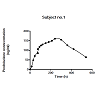
 Subject no.1 was arbitrarily chosen among the ten subjects participating in the current study, to show an example of the results obtained. Therefore, the results of subject no.1 were described in detail in the text bellow. Figure 1 showed the observed plasma concentration versus time profile of prednisolone and the description of the observed profile with the model of the subject’s dynamic system H. Analogous results to those obtained for subject no.1 were obtained for all subjects participating in the current study (Table 3).
Mathematical Model of Pharmacokinetic Behavior of Orally Administered Prednisolone in Healthy Volunteers
Maria Durisova*
Department of Pharmacology of Inflammation, Institute of Experimental Pharmacology and Toxicology, Slovak Academy of Sciences, Bratislava 841 04, Slovak Republic*Address for Correspondence: Maria Durisova, Department of Pharmacology of Inflammation, Institute of Experimental Pharmacology and Toxicology, Slovak Academy of Sciences, Bratislava 841 04, Slovak Republic, Tel/Fax: 00421254775928; E-mail: Maria.Durisova@savba.sk
Citation: Durisova M. Mathematical Model of Pharmacokinetic Behavior of Orally Administered Prednisolone in Healthy Volunteers. J Pharmaceu Pharmacol. 2014;2(2): 5.
Copyright © 2014 Durisova M. This is an open access article distributed under the Creative Commons Attribution License, which permits unrestricted use, distribution, and reproduction in any medium, provided the original work is properly cited
.Journal of Pharmaceutics & Pharmacology | ISSN: 2327-204X | Volume: 2, Issue: 2
Submission: 13 August 2014 | Accepted: 09 October 2014 | Published: 14 October 2014
Abstract
The objective of the current study was to develop mathematical models that described the pharmacokinetic behavior of prednisolone in healthy subjects after the oral administration of prednisolone. The current study is a companion piece of a related Leclercq and Copinsehi prednisolone study published in the February 1974 issue of the Journal of Pharmacokinetics and Biopharmaceutics. In the study cited here, plasma concentration versus time profiles of prednisolone were determined, however, no mathematical models of the pharmacokinetic behavior of prednisolone were developed. Therefore in the current study, mathematical models of the pharmacokinetic behavior of prednisolone were developed using mathematical and computational tools from the theory of dynamic systems. The current study demonstrated the successful use of mathematical and computational tools from the theory of dynamic systems in pharmacokinetic modeling.Key words
Keywords: Prednisolone; Oral administration; Mathematical modelIntroduction
Prednisolone is commonly used to treat patients with asthma [1], rheumatoid arthritis [2], hyperemesis gravidarum [3], reactive amyloidosis [4], pulmonary veno-occlusive disease [5], and many other diseases, including inflammatory bowel disease [6]. After prednisolone administration, concentrations of prednisolone in plasma were determined; however no mathematical models of the pharmacokinetic behavior 87-106 of prednisolone were developed. Ten normal male volunteers, aged 21-51 years (mean 29), weighing 87-106% (mean 97%) of their ideal weight [7], were given prednisolone on two occasions separated by a 3-day interval The current study is a companion piece of the related study by Leclercq and Copinsehi [8]. Therefore, mathematical models of the pharmacokinetic behavior of prednisolone after oral administration of prednisolone to healthy subjects were developed here. Mathematical and computational tools from the theory of dynamic systems were used in the current study, see for example the following papers [9-20] and references therein. The same tools were used in the current study.Methods
The data from the published article by Leclercq and Copinsehi [8] were used. In the study by Leclercq R. and Copinsehi G. [8], prednisolone was orally administered to ten fasting healthy male volunteers aged 21-51 years (mean 79), weighting 87-106 % (mean 97%) of their ideal weight [7] at a dose of 20 mg. Blood samples were taken 15, 30, 45, 60, 75, 90, 105, 120, 150, 180, 210, 240, 300, 360, 420, 540 min after prednisolone administration.For modeling purposes the same method as that used previously [10-14] was used. The modeling method can be briefly described as follows: In the first step, the dynamic systems, denoted by H, were defined. In the second step, the dynamic systems H, were used to mathematically describe dynamic aspects of the pharmacokinetic behavior of prednisolone in the subjects [20,21]. In the third step, the transfer functions, denoted by H(s), of the dynamic systems H, were derived using prednisolone data [7]. After the definition, the dynamic systems H, were described with transfer functions H(s), where S is the Laplace variable [9-19]. The transfer functions H(s), were derived as follows:
In Eq. (1), C(s) is the Laplace transform of the mathematical representation of the plasma concentration-versus-time profile of prednisolone, I(s) is the Laplace transform of the mathematical representation of the oral administration of prednisolone, and the lower-case letter “ S ” denotes the complex Laplace variable, see for example the following studies [10-18]. These assumptions were made for the current study: a) the dynamic systems H started with zero initial conditions, b) the pharmacokinetic processes occurring in the body after prednisolone administration were linear and time-invariant, c) prednisolone concentrations were the same throughout the subsystems, d) no barriers to the distribution (or elimination) of prednisolone existed.For modeling purposes, the software named CTDB [11], and the transfer function model HM (s) described by the Eq. (2), were used:
On the right-hand-side of Eq. (2) is the Padé approximant to the model transfer function HM(S), G is an estimator of the model parameter called the gain of the dynamic system H, a1,....an, b1,......bm, are the additional model parameters, and n is the highest degree of the nominator polynomial, m is the highest degree of the denominator polynomial, where n < m see for example the following studies [10-15].
In the next step the transfer functions H(s) were converted into equivalent frequency response functions, denoted by F(iωj). In the fourth step, the non-iterative method published previously [22] was used to determine models of frequency response functions FM(iωj) and point estimates of the parameters of the model frequency response functions FM(iωj) in the complex domain. The model of the frequency response function FM(iωj) used in the current study is described by the following equation:
Analogously as in Eq. (2), in Eq. (3), n is the highest degree of the numerator polynomial of the model frequency response function FM(iωj), m is the highest degree of the denominator polynomial of the model frequency response function FM(iωj), i the imaginary unit, and ω is the angular frequency. In the fifth step, the model frequency response functions FM(iωj) were refined, using the Monte-Carlo and the Gauss-Newton method in the time domain. In the fifth step, the Akaike information criterion was used to discriminate among the models of frequency response functions FM(iωj) of different complexity and to select the best models frequency response function FM(iωj) with the minimum score of the Akaike information criterion [23]. In the final step, 95 % confidence intervals for each parameter of the final models FM(iωj) were determined.
On the basis of the models developed, the following primary pharmacokinetic variables were determined: The time of occurrence of the maximum observed plasma concentration of prednisolone, denoted by tmax, the maximum observed plasma concentration of prednisolone, denoted by Cmax, the plasma elimination halftime of prednisolone, denoted by t1/2 , the area under the plasma concentration versus time curve from time zero to infinity, denoted by, AUC0−∞,and total body clearance of prednisolone, denoted by CI.
The transfer function model HM(S) and the frequency response function model FM(iωj) are implemented in the computer program CTDB [11]. A demo version of the computer program CTDB is available for downloading from the web site: http://www.uef.sav.sk/advanced.htm.
Results
The final third-order model of FM(iωj) selected with the Akaike criterion is described by Eq. (4): This model provided good fit to the prednisolone concentration data in all subjects participating in the current study. Estimates of model parameters a0, a1, b1, b2, b3 are listed in Table 1. Model-based estimates of primary pharmacokinetic variables included: time of occurrence of the maximum observed plasma concentration of prednisolone, denoted by tmax, the maximum observed plasma concentration of prednisolone, denoted by Cmax, the plasma elimination half-time of prednisolone, denoted by t1/2, the area under the plasma concentration versus time curve from time zero to time infinity, denoted by, AUC0-∞, and total body clearance of prednisolone, denoted by CI. The primary pharmacokinetic variables are listed as means with SDs in Table 2.
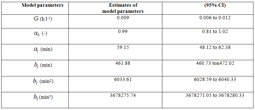
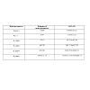
Table 1: Parameters of the third-order model of the dynamic system describing the pharmacokinetic behavior of orally administered prednisolone to the subject no.1
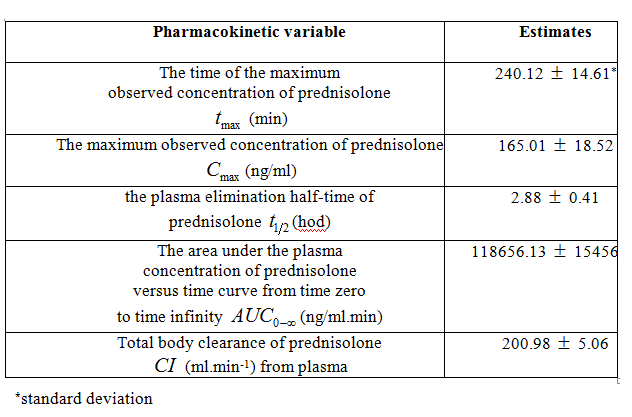
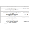
Table 2: Pharmacokinetic variables of orally administered prednisolone to the subject no.1.
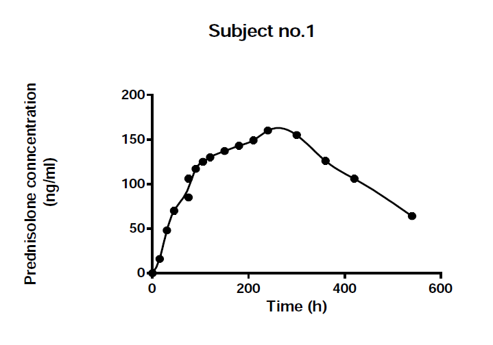
Figure 1: Observed venous plasma concentration versus time profile of prednisolone and the description of the observed profile with the model of the subject’s dynamic system which mathematically described the dynamic aspects of pharmacokinetic behavior of prednisolone.
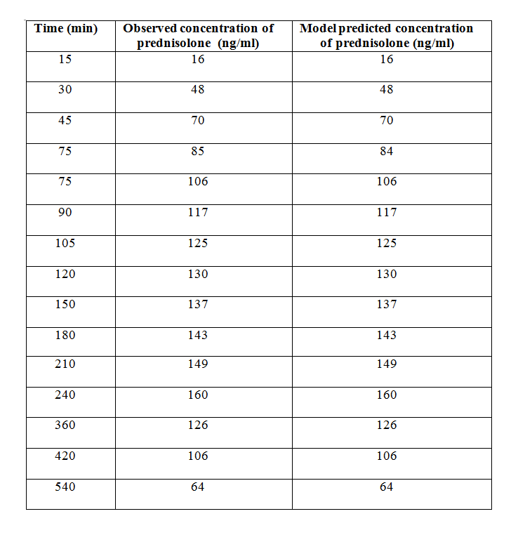
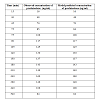
Table 3: Observed and model predicted blood concentrations of prednisolone in the subject no.1.
Discussion
The dynamic systems used in the current study were mathematical objects, without any physiological relevance. They were employed to model dynamic aspects [17-21] of the pharmacokinetic behavior of prednisolone in healthy subjects after oral administration of prednisolone at a dose of 20 mg. The development of the mathematical models used in the current study has been described in detail previously [10-16].As in previous studies, authored or co-authored by the author of the current study [10-16], the development of mathematical models of the dynamic systems H, was based on the measured input(s) and output(s) of the dynamic systems H. Generally, if a dynamic system is modeled using the transfer function models HM(S), as it was the case in the current study, then the accuracy of the model depends in large part on the degrees of the polynomials of the transfer function models HM(S) used to fit the data [22].
Each transfer function H(s) was defined as the ratio between the Laplace transform of the mathematical representation of the plasma concentration versus time profile of prednisolone, denoted by C(s), and the Laplace transform of the mathematical representation of the oral administration of prednisolone, denoted by I(s), see Eq. (2). The parameter gain is also called gain coefficient, or gain factor. According to the theory of dynamic systems, the parameter gain is defined as a relationship between the magnitude of an output of the dynamic system to a magnitude of an input to the dynamic system in steady state.
As it follows from the theory of dynamic systems, the parameter gain of a dynamic system is a proportional value that shows the relationship between the magnitude of an output to a magnitude of an input of a dynamic system at steady state. The pharmacokinetic meaning of the parameter gain depends on the nature of the dynamic system; see for example studies available on the Internet: http://www.uef.sav.sk/advanced.htm. The non-iterative method published in the study [22] and used in the current study is capable of providing quick identification of a structure of a model frequency response.
The reason for conversion of HM(S) into FM(iωj) was that "S" in HM(S) is a complex Laplace variable (see Eq. (2)), while the angular frequency ω is a real variable (see Eq. (4)).
Prednisolone exhibits nonlinear pharmacokinetics mainly due to prednisolone nonlinear protein binding. The dose dependent pharmacokinetics of prednisolone has been observed in several studies within various species [24-39]. However, for one oral dose of prednisolone (20 mg), the linear mathematical models developed in the current study sufficiently approximated the dynamic aspects of the pharmacokinetic behavior of prednisolone.
The results obtained in the current study have not been validated sufficiently to be used for clinical patient care. Their validity can be verified in clinical investigations among patients; consequently practical utilization of the results obtained in the current study lies far in the future. The idea behind the model described by Eq. (2) is not new in pharmacokinetics. See the following studies [9-18].
The current study showed the successful use of mathematical and computational tools from system engineering in mathematical modeling of dynamic systems. Frequency response functions are complex functions, with real and imaginary components, therefore, the modeling methods used to model frequency response functions are computationally intensive, and modeling is performed in the complex domain. Moreover, the methods considered here require at least partial knowledge of the theory of dynamic system, and an abstract way of thinking about the dynamic system under study.
The principal difference between traditional pharmacokinetic modeling methods and modeling methods that use of mathematical and computational tools from the theory of dynamic systems, is as follows: the former methods are based on modeling plasma (or blood) concentration versus time profiles of drugs, however the latter methods are based on modeling relationships between a mathematically represented drug administration and a mathematically represented resulting plasma (or blood) concentration-time profile of the drug administered [10-16]. See for example the studies available at http://www.uef.sav.sk/advanced.htm. The computational and modeling methods that use computational and modeling tools from the theory of dynamic systems can be used for example for adjustment of drug administration aimed at achieving and then maintaining required drug concentration–time profiles in patients. The methods considered here can be used for safe and cost-effective individualization of drug dosing by computer-controlled infusion pumps. This is very important for example for administration of Factor VIII to hemophilia patients, as exemplified in the study [14].
The advantages of the model and modeling method used in the current study are evident here: The models developed and used overcome one of the typical limitations of compartmental models: For the development and use of the models presented here, an assumption of well-mixed spaces in the body is not necessary. The basic structure of the models developed and used is and broadly applicable and therefore it can be used in mathematical modeling different dynamic systems in the field of pharmacokinetics and in many other fields. From a point of view of pharmacokinetic community, an advantage of the models developed and used is that the models considered here emphasize dynamical aspects of the pharmacokinetic behavior of a drug in a human body. The method used can be easily generalized and can be further employed in several studies.
Conclusion
The models developed and used in the current study successfully described the pharmacokinetic behavior of prednisolone after oral administration at a dose of 20 mg to healthy subjects. The modeling method used is comprehensive and flexible and thus it can be applied to a broad range of dynamic systems in the field of pharmacokinetics and in many other fields. The current study presented a new view on “old” principles associated with the pharmacokinetic behavior of prednisolone in a human body. In addition, it presented another attempt to visualize the successful use of mathematical and computational tools from the theory of dynamic systems in pharmacokinetic modeling. For the previous attempts, please visit http://www.uef.sav.sk/advanced.htm. The author conclude that the current study showed that an integration of pharmacokinetic and bioengineering approaches is a good and efficient way to study processes in pharmacokinetics. The reason for this is that such integration combines mathematical rigor with biological insight.Acknowledgements
The author gratefully acknowledges the financial support from the Slovak Academy of Sciences in Bratislava, Slovak Republic.References
- Nelson-Piercy C (2001) Asthma in pregnancy. Thorax 56: 325-328.
- Ostensen M (2001) Drugs in pregnancy. Rheumatological disorders. Best Pract Res Clin Obstet Gynaecol 15: 935-969.
- Nelson-Piercy C, Fayers P, de Swiet M (2001) Randomised, doubleblind, placebo-controlled trial of corticosteroids for treatment of hyperemesis gravidarum. Bjog 108: 9-15.
- Ahlmen M, Ahlmen J, Svalander C, Bucht H (1987) Cytotoxic drug treatment reactive amyloidosis in rheumatoid arthritis with special reference to renal insufficiency. Clin Rheumatol 6: 27-38.
- Kano G, Nakamura K, Sakamoto I (2014) Pulmonary veno-occlusive disease in an 11-year-old girl: Diagnostic pitfalls. Pediatr Int 56: 119-122.
- Naftali T, Mechulam R, Lev LB, Konikoff FM (2014) Cannabis for inflammatory bowel disease. Dig Dis 32: 468-474.
- Lorentz FH (1929) Ein neuer Constitution index. Klin Wschr 8: 348-351.
- Leclercq R, Copinsehi G (1974) Patterns of plasma levels of prednisolone after oral administration in man. J Pharmacokinet Biopharm 2: 175-187.
- van Rossum JM, de Bie JE, van Lingen G, Teeuwen HW (1989) Pharmacokinetics from a dynamical systems point of view. J PharmacokinetBiopharm 17: 365-392.
- Verotta D (1996) Concepts, properties, and applications of linear systems to describe distribution, identify input, and control endogenous substances and drugs in biological systems. Crit Rev Biomed Eng 24: 73-139.
- Dedík L, Ďurišová M (2004) Advanced system approach based methods for modeling biomedical systems. In: International Conference of Computational Methods in Sciences and Engineering (ICCMSE 2004). Simos T, Maroulis G (Editors). Koninklijke Brill NV: Leiden, Netherlands: 136-139.
- Dedík L, Ďurišová M (1996) CXT-MAIN: A software package for determination of the analytical form of the pharmacokinetic system weighting function. Comput Methods Programs Biomed. 51: 183-192.
- Ďurišová M, Dedík L (1997) Modeling in frequency domain used for assessment of in vivo dissolution profile. Pharm Res 14: 860-864.
- Ďurišová M, Dedík L (2002) A system-approach method for the adjustment of time-varying continuous drug infusion in Individual patients: A simulation study. J Pharmacokinet Pharmacodyn 29: 427-444.
- Ďurišová M, Dedík L (2005) New mathematical methods in pharmacokinetic modeling. Basic Clin Pharmacol Toxicol 96: 335-342.
- Ďurišová M, Dedík L, Kristová V, Vojtko R (2008) Mathematical model indicates nonlinearity of noradrenaline effect on rat renal artery. Physiol Res 57: 785-788.
- Ďurišová M (2014) The use of methods based on the theory of dynamical systems for mathematical modeling in biomedical research. Research 1: 732.
- Ďurišová M (2014) A physiological view of mean residence times. Gen Physiol Biophys 33: 75–80.
- Weiss M, Pang KS (1992) Dynamics of drug distribution. I. Role of the second and third curve moments. J Pharmacokinet Biopharm 20: 253-278.
- Xiao H, Song H, Yang Q, Cai H, Qi R, et al. (2012) A prodrug strategy to deliver cisplatin (IV) and paclitaxel in nanomicelles to improve efficacy and tolerance. Biomaterials 33: 6507–6519.
- Ramsey HH, Levine J, Kennedy-Stoskopf S, Taylor SK, Shea D, et al. (2009) Development of a Dynamic Pharmacokinetic Model to estimate bioconcentration of xenobiotics in earthworms. Environ Model Assessment 14: 411-418.
- Levy EC (1959) Complex curve fitting. IRE Trans Automat Contr AC 4: 37-43.
- Akaike H (1974) A new look at the statistical model identification. IEEE Trans Automat Contr 19: 716-723.
- Boudinot FD, Jusko WJ (1986) Dose-dependent pharmacokinetics of prednisolone in normal and adrenalectomized rats. J Pharmacokinet Biopharm 14: 453-467.
- Huang ML, Jusko WJ (1990) Nonlinear pharmacokinetics and interconversion of prednisolone and prednisone in rats. J Pharmacokinet Biopharm 18: 401–421.
- Pickup ME, Lowe JR, Leatham PA, Rhind VM, Wright V (1977) Dose dependent pharmacokinetics of prednisolone. Eur J Clin Pharmacol 12: 213-219.
- Rose JQ, Yurchak AM, Jusko WJ (1981) Dose dependent pharmacokinetics of prednisone and prednisolone in man. J Pharmacokinet Biopharm 9: 389-417.
- Wald JA, Law RM, Ludwig EA, Solan RR, Middlketon E, et al. (1992) Evaluation of dose-related pharmacokinetics and pharmacodynamics of prednisolone in man. J Pharmacokinet Biopharm 20: 567-589.
- Jones RT, Evans W, Mersfelder TL, Kavanaugh K (2014) Rare red rashes: A Case Report of Levetiracetam-Induced Cutaneous Reaction and Review of the Literature. Am J Ther.
- Osmanağaoğlu MA, Kesim M, Yuluğ E, Menteşe A, Karahan CS (2012) The Effect of High Dose Methylprednisolone on Experimental Ovarian Torsion/Reperfusion Injury in Rats. Geburtshilfe Frauenheilkd 72: 70-74.
- Ma XR, Quyang TX, Ma YT, Chen WY, Chang ML (2014) Successful treatment of Kimura’s disease with leflunomide and methylprednisolone: a case report. Int J Clin Exp Med 7: 2219-2222.
- Burki TK (2014) Methylprednisolone in patients with cancer using opioids. Lancet Oncol 15: e370.
- Miller MW, Agrawal Y (2014) Intratympanic Therapies for Menière‘s disease. Curr Otorhinolaryngol Rep 2: 137-143.
- Fytili C, Bourmia VK, Pentazos G, Kokkinos A (2014) Multiple cranial nerve palsies in giant cell arthritis and response to cyclophosphamide: a case report and review of the literature. Rheumatol Int.
- Rosado IR, Lavor MS, Alves EG, Fukushima FB, Oliveira KM, et al. (2014) Effects of methylprednisolone, dantrolene, and their combination on experimental spinal cord injury. Int J Clin Exp Pathol 7: 4617-4626.
- Siegel RA (1986) Pharmacokinetic transfer functions and generalized clearances. J Pharmacokin Biopharm 14: 511-521.
- Segre G (1988) The sojourn time and its prospective use in pharmacology. J Pharmacokinet Biopharm 16: 657-666.
- Yates JW (2006) Structural identifiability of physiologically based pharmacokinetic models. J Pharmacokinet Pharmacody 33: 421-439.
- Rescigno A (2010) Compartmental analysis and its manifold applications to pharmacokinetics. AAPS J 12: 61-72.