
Journal of Pharmaceutics & Pharmacology
Download PDF
Research Article
Address for Correspondence:Maria Durisova, Department of Pharmacology of Inflammation, Institute of Experimental Pharmacology and Toxicology, Slovak Academy of Sciences Bratislava, Slovak Republic,; E-mail: Maria.Durisova@savba.sk
Citation: Durisova M. Another Example of a Successful Use of Computational and Modeling Tools from the Theory of Dynamic Systems in Pharmacokinetic Modeling. J Pharmaceu Pharmacol. 2015;3(1): 3.
Copyright © 2015 Durisova M. This is an open access article distributed under the Creative Commons Attribution License, which permits unrestricted use, distribution, and reproduction in any medium, provided the original work is properly cited.
Journal of Pharmaceutics & Pharmacology |ISSN: 2327-204X| Volume: 3, Issue: 1
Submission: 19 November 2014 | Accepted: 21 January 2015 | Published: 26 January 2015
Another Example of a Successful Use of Computational and Modeling Tools from the Theory of Dynamic Systems in Pharmacokinetic Modeling
Maria Durisova*
- Department of Pharmacology of Inflammation, Institute of Experimental Pharmacology and Toxicology, Slovak Academy of Sciences Bratislava, Slovak Republic
Address for Correspondence:Maria Durisova, Department of Pharmacology of Inflammation, Institute of Experimental Pharmacology and Toxicology, Slovak Academy of Sciences Bratislava, Slovak Republic,; E-mail: Maria.Durisova@savba.sk
Citation: Durisova M. Another Example of a Successful Use of Computational and Modeling Tools from the Theory of Dynamic Systems in Pharmacokinetic Modeling. J Pharmaceu Pharmacol. 2015;3(1): 3.
Copyright © 2015 Durisova M. This is an open access article distributed under the Creative Commons Attribution License, which permits unrestricted use, distribution, and reproduction in any medium, provided the original work is properly cited.
Journal of Pharmaceutics & Pharmacology |ISSN: 2327-204X| Volume: 3, Issue: 1
Submission: 19 November 2014 | Accepted: 21 January 2015 | Published: 26 January 2015
Abstract
The objective of the current more or less theoretical study was to provide another example of a successful use of computational and modeling tools from the theory of dynamic systems in pharmacokinetic modeling. The tools considered here, were used to develop mathematical models of the pharmacokinetic behavior of ethanol following its intravenous infusion to dogs. The data used in this study, were drawn from the study: (Rheingold JL, Lindstrom RE, Wilkinson PK, A new blood-flow pharmacokinetic model for ethanol. J Pharmacokinet Biopharm. 1981; 9:3261-3278). The method developed by Dedík and Ďurišová was employed for modeling purposes. A description of the method considered here has been published in the study: Dedík L, Ďurišová M. (Advanced system approach based method for modeling biomedical systems. In International Conference of Computational Methods in Sciences and Engineering, ICCSE 2004. T. Simos, G. Maroulis (Eds). Koninklijke Brill NV: Leiden, Netherlands 2004, 136-139). As it follows from the results obtained, the mathematical models developed successfully described the pharmacokinetic behaviorof infused ethanol in all dogs studied. The modeling method used inthe current more or less theoretical study is an alternative modeling method to modeling methods frequently used in pharmacokinetics.Introduction
The current study is related to the study by Rheingold et al. describing a new blood-flow pharmacokinetic model for ethanol, andpublished in the March 1981 issue of Journal of Pharmacokinetics and Biopharmaceutics [1]. Using the data published in the studycited here, another example of a successful use of computational and modeling tools from the dynamic systems theory in pharmacokinetic modeling was provided in this more or less theoretical study (thereafter only in the current study). The previous examples can be found in the full-text articles available free of cost at the Internetaddress: http://www.uef.sav.sk/advanced.htm.A short description of the study [1] is as follows: 1) ethanol was administered to healthy full-grown mongrel dogs weighing 18-31 kg by an intravenous infusion over 10 minutes; 2) two different ethanol doses (0.13 and 0.26 g/kg) were used; 3) the ethanol infusion was performed with indwelling catheters in the hepatic artery, hepatic vein, portal vein, and femoral artery; 4) following the ethanol infusion concentrations of ethanol in the femoral artery and femoral vein were determined; 5) to develop mathematical models of thepharmacokinetic behavior of ethanol, the modeling program named CSMP (Continuous System Modeling Program) [2] and a modeling method frequently used in pharmacokinetics were employed. In thecurrent study, mathematical models of the pharmacokinetic behavior of the infused ethanol in dogs were developed, using an alternative modeling method to that used in the study [1], i.e. the modeling method based on the theory of dynamic systems and the computer program named CTDB (Complex Tools Data Base) [3]. A demo version of CTDB is available free of cost on the Internet address:http://www.uef.sav.sk/advanced.htm.
Dynamic processes associated with the fate and disposition of an administered drug in a human and/or animal body are influenced not only by various dynamic interactions between the drug administered and physiological environment but also by various factors, see for example the following studies [3,10]. Therefore, several articles described investigations of dynamic processes associated with fate and disposition of administered drugs in a human or animal body using computational and modeling tools from the theory of dynamic systems, see for example the following studies [3,8]. A few examples describing the successful use of computational and modeling tools from the theory of dynamic systems in pharmacokinetic modeling can be found in the full-text articles available free of cost on the Internet address: http://www.uef.sav.sk/advanced.htm.
Materials and Methods
The modeling of the pharmacokinetic behavior of ethanol in the dogs was performed in the following way: In the first step, ADME related dynamic systems, denoted by H, were defined using transfer functions, denoted by H(s), in the Laplace domain. In Eq. (1), s is the Laplace variable, Cethanol(s) is the Laplace transform of the concentration-time profile of ethanol in the femoral artery, and/or the femoral vein, and Iethanol(s) is the Laplace transformof the ethanol infusion. (ADME is an acronym frequently used in pharmacokinetics and pharmacology, for absorption, distribution, metabolism, and excretion, of a drug administered). In the following text the ADME related dynamic systems H were simply called the dynamic systems H. Mathematical models of the dynamic systems H were developed using the method described previously [3,8]. A shortdescription of the modeling method used is as follows: For modeling purposes, the transfer function model HM(S), described by the Eq. (2),was used:
On the right-hand-side of Eq. (2) is the Padé approximant to the model transfer function HM(S), G is an estimator of the model parameter called the gain of the dynamic system H, a1, …an, b1, … bm are the additional model parameters, and n is the highest degree of the nominator polynomial, m is the highest degree of the denominator polynomial, where n < m [3-7].
In the second step, the transfer functions H(s) were converted into equivalent frequency response functions, denoted by F(ij) in the complex domain [3-7]. In the third step, the non-iterative method published previously [11] was used to determine models of frequency response functions FM(iωj) and point estimates of the parameters of the model frequency response functions FM(ij) in the complex domain. The model of the frequency response function FM(iωj) used in the current study is described by the following equation:
Analogously as in Eq. (2), n is the highest degree of the numerator polynomial of the model frequency response function FM(iωj), m is the highest degree of the denominator polynomial of the model frequency response function FM(iωj), i the imaginary unit, and ω is the angular frequency in Eq.(3). In the next step, the model frequency response functions FM(iωj) were refined, using the Monte-Carlo and the Gauss-Newton method in the time domain. In the fifth step, the Akaike information criterion was used to discriminate among the models frequency response functions FM(iωj) of different complexity and to select the best models frequency response function FM(iωj)[12]. In the final step, 95 % confidence intervals for each parameter of the final models FM(iωj were determined.
Results
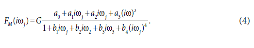
The results obtained for dog no.1, were arbitrarily chosen, to show the results obtained. The final fourth-order model of FM(iωj) selected with the Akaike criterion is described by Eq. (4): This model provided good fit to the ethanol concentration data in all dogs studied. Estimates of model parameters a0, a1, a2, a3, b1, b2, b3 and b4 were:
a0=.99±0.09, a1=.99±0.09, a2=60.51±2.35 (min2), a3=60.51±7.83 (min3), b1=472.8±99.2 (min), b2=72.8±6.5 (min2), b3=46787.8±323.5 (min2), b4=98568.8±125.8 (min4).
Model-based estimates of primary pharmacokinetic variables included: the distribution volume of ethanol, the rate of elimination of ethanol, the time of occurrence of the maximum observed plasma concentration of ethanol, the maximum observed plasma concentration of ethanol, the plasma elimination half-time of ethanol, and total body clearance of ethanol. The primary pharmacokinetic variables are listed as means with SDs in Table 1.
figure 1 shows the observed concentration-time profile of ethanol in the femoral artery, and description of the observed profile with the model of the dog’s dynamic system H. Analogous results were obtained for all dogs studied.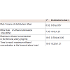
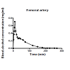
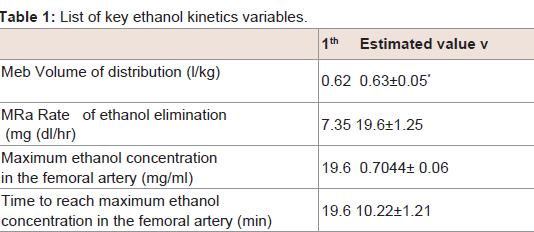
Table 1: List of key ethanol kinetics variables.
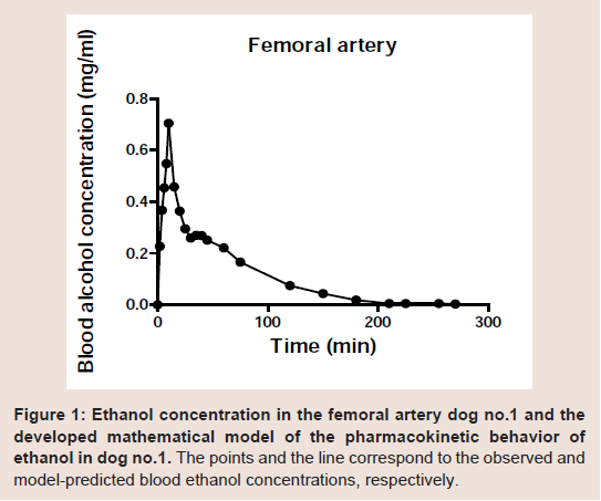
Figure 1:Ethanol concentration in the femoral artery dog no.1 and the developed mathematical model of the pharmacokinetic behavior of ethanol in dog no.1. The points and the line correspond to the observed and model-predicted blood ethanol concentrations, respectively.
Discussion
Many examples of analyses of the pharmacokinetic behavior of ethanol can be found by a MEDLINE search. Therefore the current study was not aimed at investigating the pharmacokinetic behavior of ethanol. In contrast, the current study was aimed at providing another example of a successful use of computational and modeling tools from the theory of dynamic systems in pharmacokinetic modeling. As it follows from the results obtained, that the alternative modeling method used in the current study was appropriately employed, because the developed mathematical models of the dynamic systems H successfully described the pharmacokinetic behavior of the infused ethanol in all dogs studied, as seen for example in the result obtained for dog. no.1 in Figure 1. As seen in Figure 1 the observed concentration-time profile of the infused ethanol in the femoral artery of dog no.1, was successfully described with the developed mathematical model of the dynamic system H. Although all results obtained were not shown, basically similar results were obtained for all dogs studied.Transfer functions are very useful tools for technical investigations. A mathematical idea to describe the pharmacokinetic behavior of an administered drug with a transfer function is not recent. A transfer function was introduced to pharmacokinetic research as early as in 1981 [13-15].
The models developed in the current study did not attempt to address all aspects of the pharmacokinetic behavior of the infused ethanol in dogs, because of the following reasons: First: it was not the aim of the current study to address all aspects of the pharmacokinetic behavior of the infused ethanol in dogs; Second: no mathematical model can describe in detail the pharmacokinetic behavior of ethanol in a dog’s body; Third: in principle, it is difficult to describe real dynamic systems precisely using mathematical equations, since the systems considered here often have an inherent uncertainty.
A review of the literature reveals that the modeling method used in the current study has not been widely utilized in pharmacokinetics as yet. Therefore, the current study was written in a language that readers not familiar with the theory of dynamic systems will easily understand.
The terminology used in the current study is commonly used in technical investigations. It is significantly different from the terminology commonly used in pharmacokinetic investigations. The fundamental difference is between the physiological nature of the information conveyed by a physiological system and the functional nature of the information conveyed by the dynamic systems used in the current study. In current study, the dynamic systems were used as working tools to mathematically represent dynamic processes [9,[10] associated with the pharmacokinetic behavior of ethanol in the dog’s body. Another difference concerns the use of the term “dynamic”. In the current study the term, dynamic “was used to indicate that the pharmacokinetic behavior of ethanol in the dog’s body is characterized by continuous changes. In contrast in pharmacokinetics the term “dynamic” is used with respect to effects of drugs. Dynamic systems used in the current study are abstract mathematical constructs, without any physiological relevance. They were used as working toolsto describe mathematically how one state of the pharmacokinetic behaviour of ethanol in a dog’s body developed into another state over the course of time. Transfer functions are the fundamental equations for analyzes of dynamical systems. They are not unknown in pharmacokinetics. They were introduced to pharmacokinetics as early as in 1981 [13-15]. Transfer functions are usually called disposition functions in pharmacokinetic research [16]. Advantages of the modeling methods based on the theory of dynamic systems over the traditional modeling methods used in pharmacokinetics were described in detail in the authors’ previous study [6].
The only and significant difference between “older dynamic system approaches” and the dynamic system approach employed in the current study is the use of the approaches considered here: “Older” dynamic system approaches are frequently used in technical investigations. In contrast, the current dynamic systems approach has been used in the pharmacokinetic investigation in the current study and in the studies previously published, available free of cost on the Internet address:http://www.uef.sav.sk/advanced.htm.
Concluding remarks
Much work remains to be done in order to further develop the modeling method used in the current study, and to implement the modeling method used in user-friendly pharmacokinetic modeling software. One of founders and of internationally known leaders in the pharmacokinetic research Professor John G. Wagner in his work [17] wrote: A modern view of pharmacokinetics must include both linear and nonlinear systems. The current study is in line with the idea presented by Professor John G. Wagner in his earlier work cited here.Acknowledgements
The author thanks to anonymous Referees for all valuable suggestions and comments which allowed to improve the manuscript and to avoid mistakes. The author also gratefully acknowledges the financial support obtained from the Slovak Academy of Sciences in Bratislava, Slovak Republic.References
- Rheingold JL, Lindstrom RE, Wilkinson PK (1981) A new blood-flow pharmacokinetic model for ethanol. J Pharmacokinet Biopharm 9: 261-278.
- Azadi G, Seward M, Larsen MU, Sharpley NC, Ttipathi A (2012) Improved antimicrobial potency through synergic action of chitosan microparticles and low electric field. Appl Biochem Biotechnol 168: 531-541.
- Dedík L, Ďurišová M (2004) Advanced system approach based methods for modeling biomedical systems. In: International Conference of Computational Methods in Sciences and Engineering (ICCSE 2004). Simos T, Maroulis G.(Eds.). Koninklijke Brill NV: Leiden, Netherlands ; 136-139.
- Dedik L, Ďurišova M (1994) Frequency response method in pharmacokinetics. J Pharmacokinet Biopharm 22: 293-307.
- Ďurišová M, Dedík L, Balan M (1995) Building a structured model of a complex pharmacodynamics system with time delays. Bull Math Biol 57: 787-808.
- Ďurišová M, Dedik L (2005) New mathematical models in pharmacokinetic modeling. Basic & Clinical Pharmacology Toxicology 96: 335-342.
- Ďurišová M, Dedík L, Kristová V, Vojtko R (2008) Mathematical model indicates nonlinearity of noradrenaline effect on rat renal artery. Physiol Res 57: 785-788.
- Ďurišová M (2014) A physiological view of mean residence times. Gen Physiol Biophys 33: 75-80.
- Verotta D (2010) Fractional dynamics pharmacokinetics-pharmacodynamic models. J Pharmacokinet Pharmacodyn 37: 257-276.
- Weiss M, Pang KS (1992) Dynamics of drug distribution. I. Role of the second and third curve moment. J Pharmacokinet Biopharm 20: 253-278.
- Levy EC (1959) Complex curve fitting. IRE Trans on Automatic Control AC 4: 37-44
- Akaike H (1974) A new look at the statistical model identification. IEEE Trans Automat Contr 19: 716-723.
- Siegel RA (1986) Pharmacokinetic transfer functions and generalized clearances. J Pharmacokin Biopharm 14: 511-521.
- Segre G (1988) The sojourn time and its prospective use in pharmacology. J Pharmacokinet Biopharm 16: 657-666.
- Smolen VF (1981) A frequency response method for pharmacokinetic model identification. In L Endrenyi 209-233.
- Spector JT, Yong R, Atenmüller E, Jabusch HC (2014) Biographic and behavioural factors are associated with music-related motor skills in children pianists. Hum Mov Sci 37: 157-166.
- Wagner JG (1973) A modern view of pharmacokinetics. J Pharmacokinet Biopharm 1: 363-401.